Natural monopoly
A natural monopoly is an economic market structure in which economies of scale are so pervasive that a single firm can supply the entire market demand at a lower long-run average total cost than two or more competing firms could achieve.
A natural monopoly is a specialized economic market structure wherein technological conditions, extreme upfront capital expenditure requirements, and pervasive economies of scale result in a subadditive cost function across the entire relevant range of market demand. In such industries, production efficiency is maximized when a single enterprise supplies the entire output of the market, as the presence of a second competing firm would duplicate massive infrastructure networks, leading to higher long-run average costs and economic waste.
Natural monopolies arise not from statutory government decrees, patents, or anti-competitive collusion, but rather from the inherent physical and mathematical properties of the production process. Classic examples include physical infrastructure utilities such as high-voltage electricity transmission grids, municipal water and sewage distribution pipes, regional natural gas pipeline networks, and freight railway roadbeds.
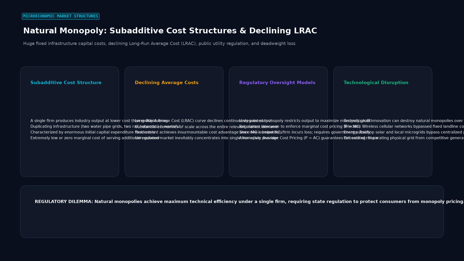 Figure: Huge fixed infrastructure capital costs, declining Long-Run Average Cost (LRAC), public utility regulation, and deadweight loss
The Mathematical Foundation: Cost Subadditivity and Declining LRAC
In microeconomic theory, the definitive criterion for a natural monopoly is cost subadditivity, formalized by economists William Baumol, John Panzar, and Robert Willig in their seminal contestable market theory.
1. The Subadditivity Condition
A cost function $C(q)$ is strictly subadditive at output level $q$ if, for any division of $q$ into $k$ distinct outputs $(q_1, q_2, \dots, q_k)$ such that $\sum_{i=1}^k q_i = q$, the cost of producing total output $q$ within a single consolidated firm is strictly less than the aggregate cost of producing those fractional quantities across separate independent firms: $$C(q) < \sum_{i=1}^k C(q_i) \quad \text{for all } q_i \ge 0 \text{ such that } \sum_{i=1}^k q_i = q$$
Even in multi-product enterprises (such as a utility supplying both peak and off-peak electricity), natural monopoly status persists so long as economies of scope combine with economies of scale to maintain overall cost subadditivity.
2. High Fixed Costs and Low Marginal Costs
Natural monopolies are characterized by an extreme asymmetry between fixed capital costs ($FC$) and marginal operating costs ($MC$):
- Fixed Infrastructure Costs ($FC$): Exceedingly large initial capital investments required to construct the distribution grid (such as digging trenches beneath municipal city streets to lay cast-iron water mains or erecting thousands of miles of high-voltage transmission pylons).
- Marginal Operating Costs ($MC$): Infinitesimal incremental costs incurred to deliver one additional unit of output through the existing grid (such as pumping one additional gallon of water through an established pipeline or transmitting one additional kilowatt-hour of electric current).
Because fixed costs are distributed across an expanding volume of output, the Long-Run Average Cost (LRAC) curve slopes continuously downward throughout the entire range of consumer market demand: $$\text{Average Total Cost (ATC)} = \frac{FC}{q} + MC$$ $$\lim_{q \to \infty} \text{ATC} = MC$$
As long as the marginal cost remains below the average cost ($MC < \text{ATC}$), the addition of each incremental consumer lowers the unit production cost for all participants in the network.
The Regulatory Dilemma: Efficiency vs. Solvency
Because a natural monopolist operates without direct market competitors, an unregulated firm would exercise market power to extract monopoly rents, creating severe economic distortions:
+------------------------+-------------------+------------------------------+
| Pricing Regime         | Market Formula    | Economic Outcome             |
+------------------------+-------------------+------------------------------+
| 1. Unregulated Private | MR = MC           | High price ($P_m$), reduced  |
|    Monopoly            | Price = $P_m$     | output ($Q_m$), maximum dead-|
|                        |                   | weight loss and excess rent  |
+------------------------+-------------------+------------------------------+
| 2. First-Best Marginal | P = MC            | Maximum allocative efficiency|
|    Cost Pricing        | Price = $P_c$     | ($Q_c$); firm incurs chronic |
|                        |                   | operating loss ($P < ATC$)   |
+------------------------+-------------------+------------------------------+
| 3. Second-Best Average | P = ATC           | Zero economic profit ($Q_r$);|
|    Cost Pricing        | Price = $P_r$     | self-financing utility with  |
|                        |                   | minimal deadweight loss      |
+------------------------+-------------------+------------------------------+
1. The Unregulated Outcome ($MR = MC$)
If left to private market incentives, the monopolist equates marginal revenue with marginal cost ($MR = MC$). The firm restricts market supply to $Q_m$ and charges price $P_m$. This results in:
- Massive transfer of consumer surplus into producer monopoly profit.
- Substantial deadweight loss (DWL), as consumers who value the service above its true marginal cost ($P > MC$) are excluded from consumption.
2. The Marginal Cost Dilemma ($P = MC$)
Allocative efficiency mandates that price equal marginal cost ($P = MC$), where society’s marginal willingness to pay matches the marginal resource cost of production (output $Q_c$).
However, because the natural monopolist operates along a downward-sloping LRAC curve, the marginal cost is strictly lower than average total cost ($MC < ATC$). $$\text{Firm Profit } \Pi = q \times (P - ATC) = q \times (MC - ATC) < 0$$
Pricing at marginal cost forces the utility into permanent negative accounting returns. Without massive ongoing public taxpayer subsidies, a private firm operating under marginal cost pricing faces immediate insolvency.
3. The Second-Best Solution: Average Cost Pricing ($P = ATC$)
To avoid public subsidies while eliminating monopoly super-profits, regulatory authorities typically enforce average cost pricing (or “fair rate of return” pricing). The regulator sets the tariff where the demand curve intersects the LRAC curve ($P_r = ATC$), ensuring that the utility earns a normal economic profit (covering operating expenses plus a fair return on invested capital) while maximizing output ($Q_r$) to the limit of financial viability.
Regulatory Frameworks and Ratemaking Methodologies
Governments employ diverse institutional mechanisms to balance capital investment incentives with consumer protection:
                  TAXONOMY OF UTILITY REGULATION REGIMES

  Cost-of-Service / Rate-of-Return               Incentive / Price-Cap (CPI - X)
  +-------------------------------------+        +-----------------------------------+
  | - Utility recovers approved costs   |        | - Tariff capped by inflation index|
  | - Guaranteed return on capital (ROR)|        | - Utility retains efficiency gains|
  | - Risk: Gold-plating / Over-invest  |        | - Risk: Service quality erosion   |
  |   (The Averch-Johnson Effect)       |        |   and deferred asset maintenance  |
  +-------------------------------------+        +-----------------------------------+
1. Rate-of-Return (Cost-of-Service) Regulation
Prevalent in the United States across state Public Utility Commissions (PUCs) and the Federal Energy Regulatory Commission (FERC), this model sets utility tariffs using the classical revenue requirement formula: $$R = O + (V - D) \times r$$ Where:
- $R$ = Total revenue requirement (the revenue the utility is legally permitted to collect).
- $O$ = Operating and maintenance expenses (fuel, labor, taxes).
- $V$ = Gross value of capital assets (utility plant in service, the “rate base”).
- $D$ = Accumulated depreciation.
- $r$ = Allowed rate of return on capital (weighted average cost of capital, WACC).
The Averch-Johnson Effect: A major flaw of rate-of-return regulation is the perverse incentive for the utility to over-capitalize. Because the firm’s dollar profit is a direct function of its invested capital rate base ($V - D$), the utility is economically incentivized to substitute capital for labor and purchase excessive, gold-plated infrastructure to inflate its guaranteed accounting profits.
2. Price-Cap Regulation (RPI - X / CPI - X)
Pioneered in the United Kingdom by economist Stephen Littlechild during the privatization of British Telecom in the 1980s, price-cap regulation severs the immediate link between a utility’s historical costs and its permitted prices. The regulator sets a multi-year price trajectory linked to consumer price inflation minus an expected productivity factor ($X$): $$\Delta P \le \text{CPI} - X$$
- If the utility improves operational efficiency and lowers unit costs faster than the $X$-factor, it retains the resulting excess profits for the duration of the regulatory cycle (typically 5 years).
- This creates strong market-like incentives to cut costs, but requires rigorous regulatory monitoring to prevent the utility from achieving savings by degrading service reliability and deferring capital maintenance.
Structural Unbundling: Separating Networks from Generation
In modern network industries, technological innovation has demonstrated that not all segments of an infrastructure supply chain are natural monopolies. Modern economic deregulation focuses on structural unbundling: segregating the non-replicable natural monopoly network (the “wires and pipes”) from the competitive market segments (generation, production, and retail billing).
                     ELECTRICITY SECTOR STRUCTURAL UNBUNDLING

  Competitive Upstream               Regulated Natural Monopoly        Competitive Downstream
  +----------------------+          +--------------------------+      +---------------------+
  | Power Generation     |          | Transmission &           |      | Retail Suppliers &  |
  | (Nuclear, Solar,     | =======> | Distribution Grid        | ===> | Energy Marketers    |
  | Wind, Gas Turbines)  |          | (Wires, Poles, Pylons)   |      | (Consumer Billing)  |
  +----------------------+          +--------------------------+      +---------------------+
  - Multiple IPP owners             - Single regulated entity         - Open retail market
  - Wholesale market bid            - Independent System Operator     - Consumer choice
1. The Electricity Model
- Generation (Competitive): Power plants (gas turbines, solar farms, wind installations) do not exhibit indefinite economies of scale. Multiple independent power producers (IPPs) compete on regional wholesale spot exchanges (such as PJM Interconnection or ERCOT).
- Transmission and Distribution (Natural Monopoly): Building parallel competing high-voltage grid lines between cities remains economically absurd. The transmission grid remains a single, highly regulated natural monopoly managed by an Independent System Operator (ISO) or Regional Transmission Organization (RTO) enforcing open-access rules.
- Retail Supply (Competitive): Multiple retail electric providers market contracts to end consumers, purchasing wholesale power and paying regulated access tariffs to the transmission grid operator.
2. Telecommunications: The Death of a Natural Monopoly
The telecommunications sector provides a historical case study in the obsolescence of natural monopolies through technological disruption:
- Throughout the twentieth century, AT&T (the Bell System) was considered an unchallengeable natural monopoly because stringing duplicate copper wire telephone lines to every household was prohibitively inefficient.
- The advent of microwave relay links, fiber-optic long-haul transport, cellular wireless communications, and satellite broadband (Starlink) eliminated the natural monopoly characteristics of voice communications, culminating in the 1982 consent decree breaking up AT&T into the “Baby Bells.”
Comparative Matrix: Natural Monopoly vs. Standard Monopolies
+------------------------+-----------------------------+-----------------------------+
| Dimension              | Natural Monopoly            | Statutory / Legal Monopoly  |
+------------------------+-----------------------------+-----------------------------+
| Underlying Catalyst    | Pervasive economies of scale| Government patents, licenses|
|                        | and high fixed capital costs| copyright, or state decrees |
+------------------------+-----------------------------+-----------------------------+
| Cost Structure         | Monotonically declining     | Standard U-shaped LRAC;     |
|                        | LRAC curve ($MC < ATC$)     | costs rise at high capacity |
+------------------------+-----------------------------+-----------------------------+
| Optimal Social State   | Single producer regulated   | Multiple competing firms;   |
|                        | on rate-of-return or price  | eliminate legal barriers    |
+------------------------+-----------------------------+-----------------------------+
| Technological Threat   | Bypassing distribution grid | Patent expiration or legal  |
|                        | (e.g., rooftop solar cells) | antitrust deregulation      |
+------------------------+-----------------------------+-----------------------------+
| Examples               | Water pipes, power grids,   | Pharmaceutical patents,     |
|                        | railway track networks      | state alcohol monopolies    |
+------------------------+-----------------------------+-----------------------------+
Best Practices for Assessing Natural Monopolies
- Evaluate Distributed Alternatives: When valuing legacy utilities, institutional investors must analyze whether emerging distributed technologies (such as battery energy storage systems and distributed microgrids) are eroding the natural monopoly protection of the central transmission grid.
- Scrutinize Regulatory Rate Base Additions: Fixed income credit analysts evaluating utility bonds should track rate case filings before public utility commissions. Favorable approvals of capital expenditure additions to the regulated rate base directly expand the utility’s future cash flow generation.
- Audit Regulatory Capture Risks: Utility investors must examine the independence of state regulatory commissions. When regulators are overly permissive, consumer blowback can trigger sudden legislative overhauls and retroactive tariff freezes.
Frequently Asked Questions (FAQ)
What makes an industry a natural monopoly rather than an artificial monopoly?
An industry is a natural monopoly when physical production technology and massive fixed capital costs make it cheaper for a single firm to supply the entire market demand than for multiple competing firms to do so. In contrast, an artificial or statutory monopoly arises when government legal barriers, patent protections, or anti-competitive collusive behavior exclude competitors from a market that would otherwise support multiple efficient producers.
Why is marginal cost pricing problematic for a natural monopoly?
Marginal cost pricing ($P = MC$) is economically efficient because price matches the marginal resource cost of the last unit produced. However, in a natural monopoly, the average total cost is continuously falling, which mathematically means marginal cost is always lower than average total cost ($MC < ATC$). If a natural monopolist is forced to charge a price equal to marginal cost, its revenues will fail to cover its massive fixed infrastructure costs, causing the firm to suffer continuous financial losses unless supported by state subsidies.
Can a natural monopoly lose its natural monopoly status over time?
Yes. Technological innovation frequently transforms natural monopolies into competitive markets. For example, long-distance telecommunications was once an ironclad natural monopoly because duplicate physical copper wires were economically prohibitive. The development of microwave data towers, high-capacity fiber-optic cables, and mobile cellular networks eliminated the structural necessity of a single physical network, allowing vibrant multi-firm competition to emerge.
Ready to trade forex?
Open a free demo account with a regulated broker. Practice with virtual funds before risking real money.