Zero-One Integer Programming
A mathematical optimization technique where decision variables are strictly restricted to binary values of zero or one, central to quantitative capital budgeting, project selection, and combinatorial portfolio optimization.
What Is Zero-One Integer Programming?
Zero-one integer programming, also referred to as binary integer linear programming (BILP), is a specialized subfield of mathematical optimization and operations research in which all decision variables are strictly constrained to assume binary values: either zero (0) or one (1).
In quantitative finance, corporate capital budgeting, and economic planning, binary variables provide the mathematical foundation for modeling discrete “all-or-nothing” decisions:
- $x_j = 1$ denotes a decision to accept, invest, build, or execute alternative $j$.
- $x_j = 0$ denotes a decision to reject, defer, cancel, or bypass alternative $j$.
Unlike standard linear programming models where variables can take fractional continuous values (such as manufacturing 4.73 units of an industrial part or investing 12.4% of fund capital in a bond), real-world economic projects cannot be deployed in arbitrary fractions. A corporation cannot construct 40% of a pharmaceutical manufacturing facility, drill half an offshore exploratory well, or acquire 60% of an indivisible corporate software license.
By restricting variables to the set ${0, 1}$, zero-one integer programming enables executives and financial engineers to identify mathematically optimal combinations of mutually exclusive, interdependent, and resource-constrained initiatives that maximize aggregate enterprise value.
Standard Mathematical Formulation
A canonical zero-one integer programming problem is formally stated as:
$$\text{Maximize} \quad Z = \sum_{j=1}^n c_j x_j$$
Subject to structural resource constraints:
$$\sum_{j=1}^n a_{ij} x_j \le b_i \quad \text{for } i = 1, 2, \dots, m$$
With the strict binary integrality condition:
$$x_j \in {0, 1} \quad \text{for } j = 1, 2, \dots, n$$
Where:
- $x_j$ represents the binary decision variable for candidate project $j$.
- $c_j$ denotes the objective function coefficient (such as the projected Net Present Value, NPV, or economic profit of project $j$).
- $a_{ij}$ represents the consumption of resource $i$ (such as initial capital expenditure, engineering labor hours, or computing bandwidth) required by project $j$.
- $b_i$ denotes the maximum available budget or capacity limit for resource $i$.
- $m$ is the total number of resource constraints.
- $n$ is the total number of candidate projects under consideration.
Modeling Complex Logical Relationships
The true analytical power of zero-one programming lies in its capacity to translate intricate qualitative corporate decisions into linear algebraic inequalities:
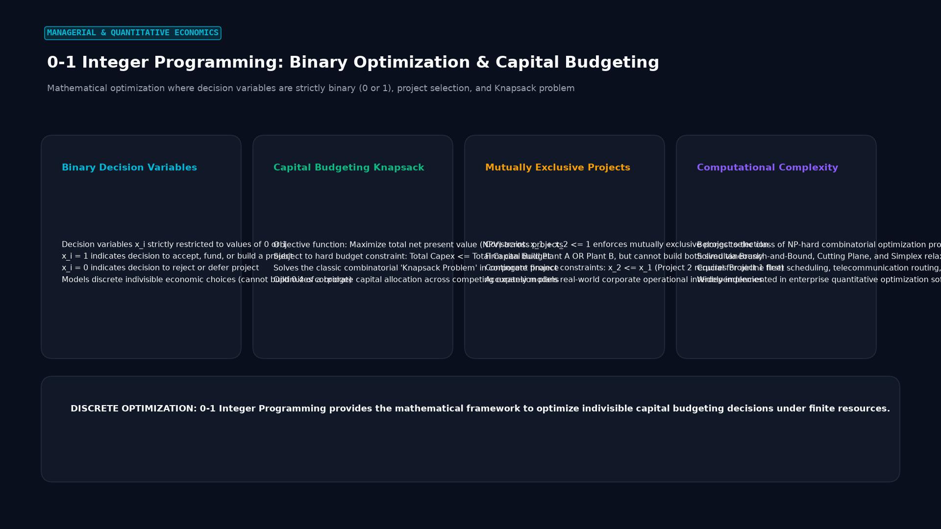 Figure: Mathematical optimization where decision variables are strictly binary (0 or 1), project selection, and Knapsack problem
1. Mutually Exclusive Projects
If a corporation is deciding between two competing ERP software platforms (Project 1 and Project 2) where implementing both is operationally impossible, the constraint is formulated as: $$x_1 + x_2 \le 1$$ If $x_1 = 1$, then $x_2$ must equal 0, ensuring that only one project is selected.
2. Contingent (Prerequisite) Projects
If an expansion of an overseas distribution hub (Project 2) can only occur if the firm first builds a local regulatory compliance office (Project 1), the relationship is modeled as: $$x_2 \le x_1 \quad \iff \quad x_2 - x_1 \le 0$$ If Project 1 is rejected ($x_1 = 0$), Project 2 is strictly barred ($x_2 \le 0 \implies x_2 = 0$). If $x_1 = 1$, Project 2 is free to be either 0 or 1 based on economic viability.
3. Corequisite (All-or-Nothing) Projects
If two technological initiatives must be implemented together or not at all: $$x_1 = x_2 \quad \iff \quad x_1 - x_2 = 0$$
The Branch-and-Bound Solution Algorithm
Because zero-one programming problems belong to the class of NP-hard combinatorial optimization problems, testing every possible combination of $n$ projects requires evaluating $2^n$ permutations. For $n = 40$, the search space exceeds one trillion candidate sets ($2^{40} \approx 1.1 \times 10^{12}$), rendering brute-force enumeration computationally impossible.
Operations researchers deploy the Branch-and-Bound algorithm, developed by Ailsa Land and Alison Doig:
                      BRANCH-AND-BOUND ENUMERATION TREE

                                  [Root Node]
                           Relax Binary: 0 <= x_j <= 1
                              Solves Continuous LP
                                       │
                     ┌─────────────────┴─────────────────┐
                     ▼                                   ▼
                Branch x_1 = 0                      Branch x_1 = 1
               Solve Sub-problem                   Solve Sub-problem
                     │                                   │
              ┌──────┴──────┐                     ┌──────┴──────┐
              ▼             ▼                     ▼             ▼
          Branch        Branch                 Branch        Branch
          x_2 = 0       x_2 = 1                x_2 = 0       x_2 = 1
             │             │                      │             │
        (Evaluated)   [PRUNED: Bound]        (Evaluated)   [INTEGER OPTIMUM]
                      Exceeds Budget                       Max NPV Found!
Operational Steps of Branch-and-Bound:
- LP Relaxation: The algorithm first drops the integrality constraint, allowing $x_j$ to take any real number between 0 and 1 ($0 \le x_j \le 1$). This relaxed problem is solved rapidly using the Simplex algorithm. The resulting objective value represents the theoretical maximum upper bound.
- Branching: If the relaxed solution yields fractional values (e.g., $x_1 = 0.65$), the algorithm partitions the problem into two non-overlapping sub-problems: one where $x_1 = 0$, and another where $x_1 = 1$.
- Bounding and Pruning: Sub-problems are evaluated sequentially. A branch is immediately “pruned” (discarded without further exploration) if:
- It violates resource constraints (infeasible).
- Its relaxed objective bound is worse than the best integer solution discovered so far.
- It yields an all-integer solution that sets a new incumbent benchmark.
Practical Case Study: Corporate Capital Rationing
An energy enterprise has allocated a strict capital expenditure (CapEx) ceiling of $50,000,000 for the upcoming fiscal year. The firm’s engineering and business development divisions present six independent capital investment proposals:
| Project ($j$) | Description | Capital Required ($a_j$) | Projected NPV ($c_j$) | Profitability Index |
|---|---|---|---|---|
| Project 1 | Solar Generation Facility | $15,000,000 | $18,000,000 | 1.20 |
| Project 2 | Pipeline Modernization | $25,000,000 | $32,000,000 | 1.28 |
| Project 3 | Deepwater Drilling Lease | $20,000,000 | $22,000,000 | 1.10 |
| Project 4 | Wind Turbine Installation | $10,000,000 | $14,000,000 | 1.40 |
| Project 5 | Carbon Capture Pilot | $8,000,000 | $9,000,000 | 1.12 |
| Project 6 | Grid Battery Storage Hub | $12,000,000 | $16,000,000 | 1.33 |
Mathematical Program: $$\text{Maximize NPV} = 18x_1 + 32x_2 + 22x_3 + 14x_4 + 9x_5 + 16x_6$$ $$\text{Subject to:} \quad 15x_1 + 25x_2 + 20x_3 + 10x_4 + 8x_5 + 12x_6 \le 50$$ $$x_1, x_2, x_3, x_4, x_5, x_6 \in {0, 1}$$
Optimization Outcome:
If a manager followed naive ranking by pure dollar NPV, they would select Projects 2 and 3, exhausting $45,000,000 of CapEx and generating $54,000,000 in aggregate NPV.
Solving the zero-one integer program yields the global mathematical optimum:
- Select Project 1 ($x_1 = 1$, Cost: $15M, NPV: $18M)
- Select Project 2 ($x_2 = 1$, Cost: $25M, NPV: $32M)
- Select Project 4 ($x_4 = 1$, Cost: $10M, NPV: $14M)
- Reject Projects 3, 5, and 6 ($x_3 = 0, x_5 = 0, x_6 = 0$)
Results:
- Total CapEx Deployed: $$15M + $25M + $10M = $50,000,000$ (100% budget efficiency)
- Total Net Present Value Created: $$18M + $32M + $14M = \mathbf{$64,000,000}$ The zero-one optimization engine unlocks $10,000,000 in incremental enterprise value compared to naive discretionary selection.
Quantitative Portfolio Management Applications
In institutional asset management, binary variables model real-world trading frictions:
- Cardinality Constraints: Mutual fund managers wishing to track an index of 1,000 stocks with a compact portfolio of exactly 50 stocks introduce binary variables ($z_i \in {0, 1}$) such that $\sum_{i=1}^N z_i \le 50$.
- Minimum Transaction Lot Sizes: Equity trading mandates often dictate that an asset manager cannot initiate a position smaller than 1.0% of fund net asset value (NAV) to prevent administrative clutter ($w_i \ge 0.01 z_i$).
- Fixed Transaction Costs: Binary variables activate fixed broker commission charges whenever trading volume occurs on an asset ($x_i = 1$ if $|\Delta w_i| > 0$).
Frequently Asked Questions
What is the difference between pure integer programming and mixed-integer programming (MIP)?
In pure zero-one integer programming, every single decision variable in the model must be a binary integer (0 or 1). In mixed-integer programming (MIP), the model contains a combination of binary variables (for discrete go/no-go decisions) and continuous real variables (for allocating dollar amounts, resource quantities, or portfolio weights).
Why can’t a financial manager simply round fractional LP solutions to the nearest integer?
Rounding fractional linear programming solutions frequently yields disastrous results. Rounding up can violate strict resource constraints (e.g., spending $52M on a $50M budget), producing an infeasible plan. Rounding down often produces severely sub-optimal results that leave significant capital unallocated and destroy millions of dollars in potential enterprise value.
What commercial solvers are used to solve zero-one programming models?
Large-scale commercial optimization problems containing hundreds of thousands of binary variables are solved using specialized commercial branch-and-cut optimization engines such as Gurobi, CPLEX, FICO Xpress, and open-source solvers like COIN-OR CBC and SCIP.
Ready to trade forex?
Open a free demo account with a regulated broker. Practice with virtual funds before risking real money.