Z-Test — Forex Dictionary Definition

What Is a Z-Test?

A z-test is a parametric statistical hypothesis test used to determine whether the difference between a sample mean and a known population mean, or between two independent sample means, is statistically significant. Under the null hypothesis ($H_0$), the calculated test statistic follows a standard normal distribution, characterized by a mean of zero and a standard deviation of one ($Z \sim \mathcal{N}(0, 1)$).

In quantitative finance, asset management, and risk modeling, z-tests serve as foundational tools for validating whether trading strategies produce genuine excess returns (alpha) or whether performance stems purely from random noise. Portfolio managers also deploy z-tests to measure whether algorithmic execution slippage deviates significantly from volume-weighted average price (VWAP) targets, evaluate credit risk rating migrations, and assess the predictive power of quantitative factors across multi-asset portfolios.

The mathematical formulation for a one-sample z-test is expressed as:

$$Z = \frac{\bar{X} - \mu_0}{\frac{\sigma}{\sqrt{n}}}$$

Where:

$\bar{X}$ represents the observed sample mean (such as the average annualized excess return of a hedge fund over $n$ periods).
$\mu_0$ denotes the hypothesized population mean under the null hypothesis (such as zero benchmark excess return).
$\sigma$ is the known population standard deviation.
$n$ equals the sample size (number of observed periods or trades).
$\frac{\sigma}{\sqrt{n}}$ represents the standard error of the mean ($SE$).

When comparing two independent sample means (for example, comparing the return distributions of two distinct algorithmic execution engines), the two-sample z-test statistic is defined as:

$$Z = \frac{(\bar{X}_1 - \bar{X}_2) - (\mu_1 - \mu_2)}{\sqrt{\frac{\sigma_1^2}{n_1} + \frac{\sigma_2^2}{n_2}}}$$

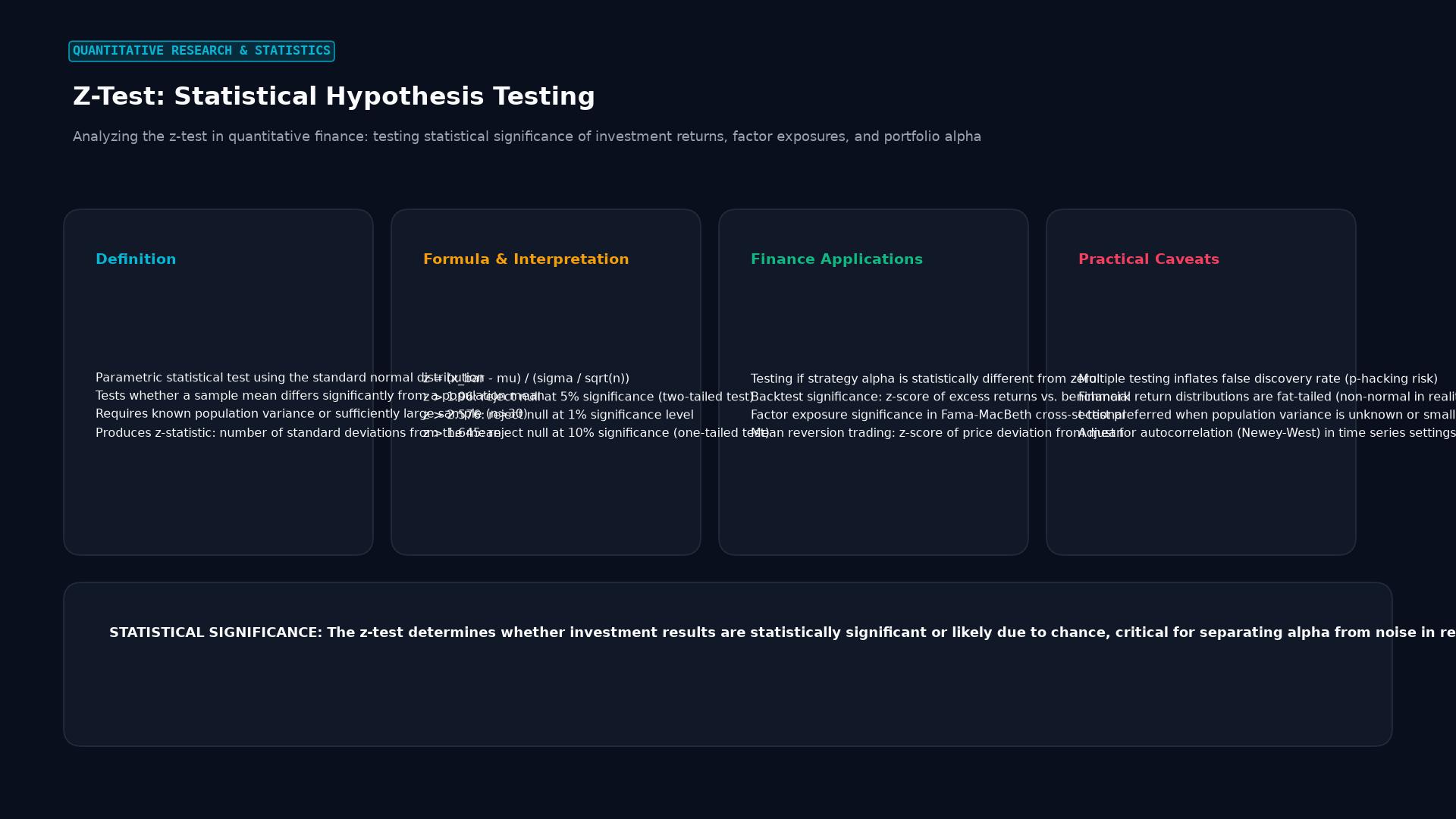Z-Test: Statistical Hypothesis Testing Figure: Analyzing the z-test in quantitative finance: testing statistical significance of investment returns, factor exposures, and portfolio alpha

Core Assumptions of the Z-Test

To ensure that inferential conclusions derived from a z-test remain statistically valid and unbiased, empirical data must satisfy three fundamental assumptions:

Known Population Variance or Large Sample Size: The classical z-test strictly requires prior knowledge of the population variance ($\sigma^2$). In real-world capital markets, true population variance is rarely known. However, invoking the Central Limit Theorem (CLT), when the sample size is sufficiently large (conventionally $n \ge 30$, and preferably $n \ge 100$ in financial time series), the sample standard deviation ($s$) converges in probability to $\sigma$, allowing the test statistic to asymptotically follow a standard normal distribution.
Independence of Observations: Individual data points must be statistically independent of one another. In financial return series, this assumption requires that returns exhibit zero serial correlation (no autocorrelation). If trading returns suffer from serial dependency (such as momentum or mean reversion), standard errors are underestimated, artificially inflating the absolute $Z$ score and generating false positive conclusions.
Normality of the Underlying Distribution: For small sample sizes, the underlying population must follow a normal distribution. While financial asset returns famously exhibit negative skewness and excess kurtosis (leptokurtosis or fat tails), large sample sizes mitigate minor departures from normality due to asymptotic convergence under the CLT.

Z-Test vs. Student’s T-Test: Key Differences

Quantitative analysts frequently choose between the z-test and Student’s t-test. The primary determinants of this choice are sample size and knowledge of the underlying population variance.

Analytical Dimension	Classical Z-Test	Student’s T-Test
Population Variance ($\sigma^2$)	Must be known, or approximated asymptotically when $n$ is large	Unknown; estimated directly via sample variance ($s^2$)
Sample Size Requirement	Typically requires $n \ge 30$ (ideally $n \ge 100$ for financial data)	Valid for small samples ($n < 30$) as well as large samples
Reference Distribution	Standard Normal distribution $\mathcal{N}(0, 1)$ with fixed tails	Student’s t-distribution with $n - 1$ degrees of freedom ($df$)
Tail Thickness	Fixed critical values ($\pm 1.96$ at 95% confidence level)	Fatter tails; critical values vary dynamically based on $df$
Primary Financial Use Case	Large-sample factor backtests, macro indicators, high-frequency trade datasets	Small-sample private equity fund returns, monthly track records of emerging managers

As sample size $n$ approaches infinity, the t-distribution converges to the standard normal z-distribution. For datasets with thousands of daily price ticks, the numerical outputs of z-tests and t-tests become virtually identical.

Applications in Quantitative Finance and Trading

1. Testing Portfolio Alpha Significance

When evaluating a hedge fund or systematic trading strategy, performance analysts regress fund returns against a benchmark index using the Capital Asset Pricing Model (CAPM):

$$R_{p,t} - R_{f,t} = \alpha + \beta (R_{m,t} - R_{f,t}) + \epsilon_t$$

To determine whether the manager generates authentic managerial skill rather than statistical luck, analysts set up a hypothesis test:

Null Hypothesis ($H_0$): $\alpha = 0$ (No excess return).
Alternative Hypothesis ($H_1$): $\alpha > 0$ (Manager creates positive alpha).

With a sample of $n = 120$ monthly return observations, the analyst calculates the estimated alpha ($\hat{\alpha}$) and its standard error ($SE_{\hat{\alpha}}$). The z-statistic is computed as:

$$Z_{\alpha} = \frac{\hat{\alpha} - 0}{SE_{\hat{\alpha}}}$$

If $Z_{\alpha} \ge 1.645$ (for a one-tailed test at the 5% significance level), the null hypothesis is rejected, supporting the conclusion that the fund creates statistically meaningful alpha.

2. Algorithmic Execution Slippage Analysis

Brokerage execution algorithms (such as TWAP, VWAP, and Implementation Shortfall) are audited by quantitative execution desks. An institutional desk executing 500 institutional orders per day tests whether the mean execution price deviation relative to the market benchmark is significantly different from zero. A two-tailed z-test reveals whether algorithm parameters require calibration to prevent systematic price degradation.

3. Factor Return Validation in Multi-Factor Models

Quantitative researchers constructing multi-factor equity portfolios (testing factors such as value, quality, low volatility, and momentum) calculate the cross-sectional mean return of long-short factor quintiles. Z-tests confirm whether the long-term historical factor premium is statistically distinct from zero before allocating capital to live trading models.

Step-by-Step Z-Test Execution Workflow

[Define Null & Alternative Hypotheses (H0 vs H1)]
                      │
                      ▼
[Select Significance Level (α = 0.05 or α = 0.01)]
                      │
                      ▼
[Identify Critical Values & Rejection Regions (Z_crit = ±1.96)]
                      │
                      ▼
[Compute Sample Mean (X_bar) & Standard Error (SE = σ / √n)]
                      │
                      ▼
[Calculate Empirical Z-Statistic: Z = (X_bar - μ0) / SE]
                      │
                      ▼
[Determine P-Value from Standard Normal Cumulative Distribution]
                      │
                      ▼
      ┌────────────────────────────────┐
      │   Is |Z_stat| > |Z_crit|?      │
      └────────────────────────────────┘
             │                  │
            YES                 NO
             │                  │
             ▼                  ▼
[Reject Null Hypothesis H0]   [Fail to Reject H0]
(Statistically Significant)   (Consistent with Noise)

State the Hypotheses: Formulate the null hypothesis ($H_0: \mu = \mu_0$) and the alternative hypothesis ($H_1: \mu \neq \mu_0$ for two-tailed, or $H_1: \mu > \mu_0$ for one-tailed).
Establish the Significance Level ($\alpha$): Select the maximum tolerable probability of committing a Type I error (false positive). Institutional research standards typically employ $\alpha = 0.05$ (5%) or $\alpha = 0.01$ (1%).
Determine Critical Values: For a two-tailed test at $\alpha = 0.05$, critical boundaries lie at $Z = \pm 1.96$. For a one-tailed test at $\alpha = 0.05$, the upper critical boundary is $Z = +1.645$.
Compute the Test Statistic: Calculate sample metrics and derive $Z$ using the standard formula.
Evaluate the P-Value: The p-value represents the probability of observing a test statistic as extreme as, or more extreme than, the observed value, assuming $H_0$ is true. If $p \le \alpha$, reject $H_0$.

Practical Case Study: Quantitative Momentum Strategy

A quantitative asset management firm develops a trend-following currency trading model deployed on the EUR/USD pair. Over an out-of-sample testing window spanning $n = 250$ trading days, the strategy achieves the following performance parameters:

Sample Mean Daily Return ($\bar{X}$): 0.08% (8 basis points)
Hypothesized Benchmark Mean ($\mu_0$): 0.00% (Cash return baseline)
Known Daily Standard Deviation ($\sigma$): 0.60% (60 basis points)
Sample Size ($n$): 250 daily trading sessions

The quantitative analyst conducts a one-tailed test at the $\alpha = 0.01$ significance level to verify whether the strategy produces authentic positive returns:

$H_0$: $\mu \le 0.00%$
$H_1$: $\mu > 0.00%$

Calculations:

Standard Error of the Mean: $$SE = \frac{\sigma}{\sqrt{n}} = \frac{0.60%}{\sqrt{250}} = \frac{0.0060}{15.8114} \approx 0.0003795 \ (0.03795%)$$
Empirical Z-Statistic: $$Z = \frac{\bar{X} - \mu_0}{SE} = \frac{0.08% - 0.00%}{0.03795%} \approx 2.108$$
Critical Value Evaluation: For a one-tailed test at $\alpha = 0.01$, the critical z-score is $Z_{0.01} = +2.326$. Since $Z_{calc} = 2.108 < 2.326$, the calculated statistic falls short of the strict 1% threshold. The corresponding one-tailed p-value is: $$p = 1 - \Phi(2.108) = 1 - 0.9825 = 0.0175 \ (1.75%)$$

Decision and Conclusion: At the strict 1% significance level, the firm fails to reject the null hypothesis. Although the strategy displays positive performance, there is a 1.75% probability that these gains arose purely from favorable random price fluctuations. The quantitative committee decides to expand out-of-sample data collection before deploying institutional balance sheet capital.

Pitfalls and Econometric Limitations in Finance

Applying standard z-tests to financial market data without appropriate econometric adjustments introduces severe statistical hazards:

Fat Tails and Leptokurtosis: Asset returns routinely display student-t or hyperbolic distributions with kurtosis far exceeding 3.0. Extreme market shocks occur much more frequently than standard normal probabilities predict. Relying on Gaussian critical values leads to an overestimation of statistical significance during market anomalies.
Autocorrelation (Serial Dependency): Trend-following and illiquid fixed-income returns often feature positive autocorrelation ($\rho > 0$). When consecutive observations are positively correlated, the effective sample size is smaller than the nominal count $n$. Using the standard formula underestimates the true standard error, producing artificially inflated z-scores. Analysts apply Newey-West autocorrelation-consistent standard errors to correct this distortion.
Heteroskedasticity: Financial volatility clusters dynamically over time, violating the constant variance assumption. The White heteroskedasticity-consistent covariance estimator or Generalized Autoregressive Conditional Heteroskedasticity (GARCH) modeling should be integrated prior to hypothesis testing.
Multiple Testing Bias (P-Hacking): When quants test hundreds of parameter combinations or technical indicators on historical data, standard individual z-tests inevitably produce false discoveries by pure chance. Researchers must apply Bonferroni corrections, Benjamini-Hochberg False Discovery Rate (FDR) procedures, or Harvey-Liu-Zhu hair-cut adjustments.

Frequently Asked Questions

When should a quantitative trader use a z-test instead of a t-test?

A trader should use a z-test when the population variance is known or when working with large sample sizes ($n \ge 100$ in financial time series) where sample variance provides an accurate estimate of population variance. If working with small sample sizes ($n < 30$), such as annual performance records of private equity funds or venture capital portfolios, a Student’s t-test is required because it accounts for estimation uncertainty through degrees of freedom.

What is the financial interpretation of a p-value in a z-test?

In an investment context, the p-value measures the exact probability that the observed performance (such as portfolio alpha or trading gains) could have occurred entirely by random market variation, assuming the strategy actually possesses zero true edge. A p-value of 0.02 indicates a 2% chance that purely random trading could generate returns equal to or greater than those observed.

How does autocorrelation distort the results of a z-test on financial returns?

When daily or monthly returns exhibit serial correlation, individual observations are not statistically independent. Positive autocorrelation reduces the effective degrees of freedom, causing the traditional standard error formula ($\sigma / \sqrt{n}$) to underestimate true volatility. This produces an artificially high z-statistic, leading analysts to reject the null hypothesis erroneously and attribute skill to random or correlated market noise.