Zero-Beta Portfolio
An investment portfolio constructed to have a beta coefficient of zero, meaning its returns exhibit zero covariance with the systematic market portfolio, serving as a core component of Fischer Black's Zero-Beta CAPM and quantitative market-neutral strategies.
What Is a Zero-Beta Portfolio?
A zero-beta portfolio is an equity or multi-asset investment portfolio constructed such that its overall beta coefficient relative to the broader market portfolio equals precisely zero ($\beta_p = 0$). In capital market theory and modern portfolio management, beta measures the sensitivity of an asset’s returns to fluctuations in the aggregate market benchmark (such as the S&P 500 or MSCI World Index).
Because a zero-beta portfolio possesses a beta of zero, its expected return exhibits zero statistical covariance with systematic market swings. In mathematical terms:
$$\beta_p = \frac{\operatorname{Cov}(R_p, R_m)}{\operatorname{Var}(R_m)} = 0 \quad \implies \quad \operatorname{Cov}(R_p, R_m) = 0$$
A zero-beta portfolio is not risk-free; it carries substantial unsystematic (idiosyncratic) risk. However, because its systematic risk is completely neutralized, the portfolio’s performance is driven purely by security-specific factors, managerial stock selection, or relative-value spreads, rather than the general direction of macroeconomic tides.
In academic asset pricing, the zero-beta portfolio is the intellectual cornerstone of Fischer Black’s Zero-Beta Capital Asset Pricing Model (1972). In contemporary institutional asset management, it serves as the operational template for equity market-neutral hedge funds and statistical arbitrage strategies seeking pure alpha.
Fischer Black’s Zero-Beta CAPM (1972)
The classical Sharpe-Lintner-Mossin Capital Asset Pricing Model (CAPM) relies on the restrictive assumption that all market participants can borrow and lend unlimited quantities of capital at a single, riskless interest rate ($R_f$). Under this assumption, all efficient portfolios lie along the Capital Market Line (CML).
Fischer Black recognized that in real-world financial markets, borrowing restrictions, margin requirements, and credit spreads prevent investors from borrowing at the risk-free rate. Black demonstrated that even in an economy without a risk-free borrowing asset, a linear asset pricing relationship still holds if one utilizes the expected return of a zero-beta portfolio ($E[R_z]$) as the reference intercept:
$$E[R_i] = E[R_z] + \beta_i \left( E[R_m] - E[R_z] \right)$$
Where:
- $E[R_i]$ is the expected return of asset or portfolio $i$.
- $E[R_z]$ is the expected return of the zero-beta portfolio.
- $E[R_m]$ is the expected return of the market portfolio.
- $\beta_i$ is the systematic risk coefficient of asset $i$.
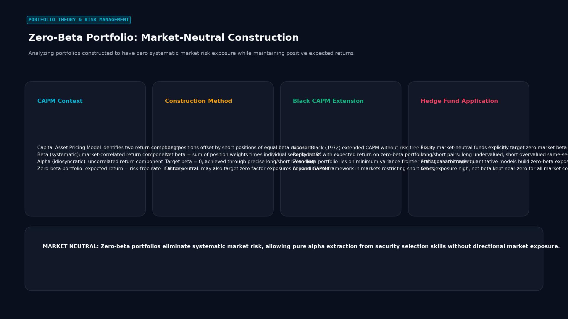 Figure: Analyzing portfolios constructed to have zero systematic market risk exposure while maintaining positive expected returns
In modern portfolio theory:
- For every efficient portfolio along the upper boundary of the Markowitz minimum-variance frontier (except the global minimum-variance portfolio), there exists a unique counterpart portfolio on the lower, inefficient half of the frontier whose returns have zero covariance with it.
- If portfolio $M$ is chosen as the market portfolio, its uncorrelated companion is the zero-beta portfolio ($Z$).
- The expected return of the zero-beta portfolio ($E[R_z]$) typically exceeds the theoretical risk-free rate ($R_f$) because it carries non-diversifiable idiosyncratic volatility, helping explain why empirical security market lines are flatter than predicted by standard CAPM.
Mathematical Construction of a Zero-Beta Portfolio
Constructing a zero-beta portfolio across $N$ assets requires determining portfolio weights ($w_1, w_2, \dots, w_N$) that satisfy two simultaneous constraints:
-
The Zero-Beta Condition: $$\beta_p = \sum_{i=1}^N w_i \beta_i = 0$$
-
The Capital Allocation Constraint: $$\sum_{i=1}^N w_i = 1 \quad \text{(For fully invested capital)}$$ $$\text{Or} \quad \sum_{i=1}^N w_i = 0 \quad \text{(For self-financing long-short arbitrage)}$$
Simplified Two-Asset Example:
Suppose a portfolio manager holds two assets:
- Asset A: High-beta technology stock with $\beta_A = 1.50$
- Asset B: Low-beta utility stock with $\beta_B = 0.50$
To build a long-only zero-beta portfolio is mathematically impossible because all weights would need to be positive, yet both betas are positive. However, introducing short selling allows the condition to be satisfied:
$$\beta_p = w_A (1.50) + w_B (0.50) = 0$$ $$w_A + w_B = 1 \implies w_B = 1 - w_A$$ $$1.50 w_A + 0.50 (1 - w_A) = 0$$ $$1.00 w_A + 0.50 = 0 \implies w_A = -0.50 \quad (-50%)$$ $$w_B = 1 - (-0.50) = +1.50 \quad (+150%)$$
By shorting $50,000 of Asset A and allocating $150,000 long to Asset B, the net capital deployed is $100,000, and the resulting portfolio beta is: $$\beta_p = (-0.50 \times 1.50) + (1.50 \times 0.50) = -0.75 + 0.75 = 0.00$$
Zero-Beta Portfolios in Modern Hedge Fund Strategies
Institutional quantitative hedge funds implement zero-beta structures through Equity Market-Neutral (EMN) strategies:
                  EQUITY MARKET-NEUTRAL (ZERO-BETA) ENGINE

  [Quantitative Stock Screener: 1,000 Equities]
                        │
         ┌──────────────┴──────────────┐
         ▼                             ▼
  [Top Decile: Undervalued]     [Bottom Decile: Overvalued]
  High Earnings Momentum        Negative Revisions
  Predicted Alpha > 0           Predicted Alpha < 0
         │                             │
         ▼                             ▼
  [Long Portfolio (+100%)]      [Short Portfolio (-100%)]
  Aggregated Beta = +1.10       Aggregated Beta = -1.10
         │                             │
         └──────────────┬──────────────┘
                        │
                        ▼
            [Combined Portfolio: Beta = 0.00]
            Net Market Exposure = $0 (Self-Financing)
            Gross Exposure = 200%
            Target: Pure Managerial Alpha
Characteristics of Institutional EMN Portfolios:
- Market Independence: During broad equity sell-offs (such as a 20% decline in the S&P 500), a true zero-beta portfolio experiences no structural downward pull. Its return is determined entirely by whether the long positions outperform the short positions.
- Factor Neutralization: Sophisticated quantitative desks neutralize both market beta and secondary risk factors (such as size, value, momentum, sector, and industry exposures), isolating pure idiosyncratic company-specific alpha.
- Leverage Application: Because daily return volatility in an unhedged zero-beta portfolio is relatively modest (typically 2% to 4% annualized), managers apply 2x to 5x balance sheet leverage through prime broker margin financing to deliver target institutional equity-like returns (8% to 12% annualized).
Practical Challenges and Quantitative Limitations
While conceptually elegant, maintaining a live zero-beta portfolio involves notable operational complexities:
- Time-Varying Beta (Beta Drift): Beta coefficients are not static physical constants; they fluctuate continuously based on market regimes, earnings cycles, and macroeconomic shocks. A portfolio calibrated to a zero beta on Monday may drift to a beta of $+0.15$ or $-0.20$ by Friday, necessitating dynamic algorithmic rebalancing.
- Estimation Error: Historical trailing betas estimated via ordinary least squares (OLS) regression are subject to sampling error. Using 60-month historical data often reflects obsolete corporate capital structures, while short-window daily betas introduce statistical noise.
- Execution Friction and Borrow Costs: Maintaining large short positions requires borrowing shares from prime brokers. Hard-to-borrow equities command substantial stock borrow fees, which erode portfolio returns over time. High rebalancing turnover also generates ongoing bid-ask spread and transaction costs.
- Liquidity Asymmetry During Crises: In liquidity crunches (such as March 2020), correlations between assets converge toward 1.0, and short positions can experience violent short squeezes while long holdings plunge, temporarily shattering zero-beta hedges.
Frequently Asked Questions
Does a zero-beta portfolio have zero risk?
No. A zero-beta portfolio eliminates only systematic (market) risk. It remains fully exposed to unsystematic (idiosyncratic) risk, such as operational failures, earnings disappointments, litigation, and management turnover among the specific companies held in the portfolio.
How does a zero-beta portfolio compare to holding cash or Treasury bills?
Treasury bills and cash possess a beta of zero because their nominal returns are fixed and immune to stock market volatility, carrying virtually zero default and price risk. A zero-beta equity portfolio also has a beta of zero, but it consists of volatile common stocks. Investors accept stock-specific volatility in a zero-beta equity portfolio in pursuit of higher expected returns (alpha) than the risk-free cash rate.
How often must a zero-beta portfolio be rebalanced?
Because individual stock betas drift as market prices change and corporate earnings evolve, institutional market-neutral funds rebalance their portfolio weights continuously or on a daily schedule. Systematic optimization algorithms monitor real-time portfolio beta and automatically submit execution orders to maintain the portfolio within tight risk tolerance bands (such as beta between -0.05 and +0.05).
Ready to trade forex?
Open a free demo account with a regulated broker. Practice with virtual funds before risking real money.