Zero-Volatility Spread (Z-Spread)
The constant yield spread added across the entire spot treasury or benchmark yield curve to discount a bond's contractual cash flows to match its dirty market price, measuring credit, liquidity, and term risk while eliminating yield curve distortion.
Zero-Volatility Spread (Z-Spread)
The zero-volatility spread (commonly abbreviated as Z-spread or yield curve spread) represents the constant basis-point spread added across the entire benchmark spot yield curve that forces the present value of a bond’s future cash flows to equal its current dirty market price. Unlike conventional yield spreads that measure the flat yield-to-maturity difference against a single benchmark bond, the Z-spread discounts every coupon payment and principal redemption against its exact point on the zero-coupon Treasury or swap curve.
In fixed-income asset management, relative-value hedge funds, and structured credit desks, the Z-spread is the premier metric for pricing vanilla corporate debt, private placements, and municipal obligations. By accounting for the unique term structure of interest rates at every cash flow horizon, it eliminates the analytical distortion inherent in upward-sloping, flat, or inverted yield curves.
                           Spot Rate Yield Curve vs. Z-Spread
  Yield (%)
     ^
     |                                                      * Cash Flow Curve (Spot + Z)
 6.0 |                                              . . . *
     |                                      . . . *       |  <--- Z-Spread (Constant Spread)
 5.0 |                              . . . *               |
     |                      . . . *                       v
 4.0 |              . . . *                               * Spot Treasury Curve
     |      . . . *
 3.0 |  . *
     +------------------------------------------------------------>
       1Y    2Y     3Y      5Y     7Y      10Y           30Y  Maturity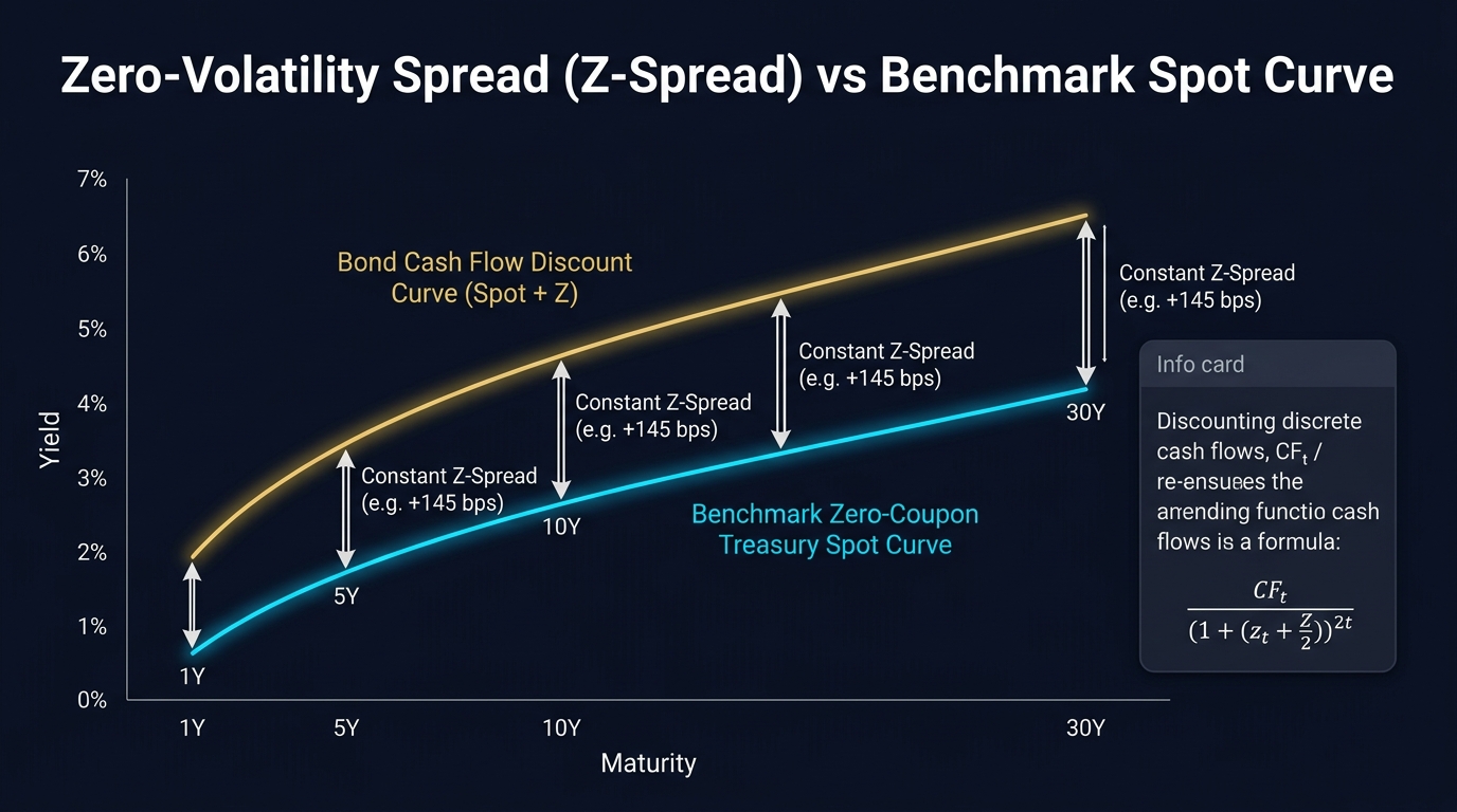
Mathematical Formulation and Discounting Mechanics
Calculating the Z-spread requires an iterative numerical algorithm (such as the Newton-Raphson method or bisection search) because the spread appears inside the denominator of every cash flow term. An analytical closed-form solution does not exist.
For a bond paying semi-annual coupons with $2n$ remaining payment periods, the market price equals the discounted sum of its discrete cash flows:
$$P_0 + AI = \sum_{t=1}^{2n} \frac{C_t}{\left(1 + \frac{r_t + Z}{2}\right)^t} + \frac{M}{\left(1 + \frac{r_{2n} + Z}{2}\right)^{2n}}$$
Where:
- $P_0$ is the clean market price of the security.
- $AI$ is the accrued interest since the last coupon date, making $P_0 + AI$ the full dirty price.
- $C_t$ represents the contractual coupon cash flow due at period $t$.
- $M$ denotes the par or redemption value paid at maturity.
- $r_t$ represents the annualized zero-coupon benchmark spot rate (derived from on-the-run Treasuries or SOFR swap rates) corresponding to the exact payment date $t$.
- $Z$ is the annualized Zero-Volatility Spread, expressed in decimal form (or converted to basis points where $1 \text{ bp} = 0.0001$).
- $t$ indexes the semi-annual compounding periods from 1 to $2n$.
Because spot rates change along the maturity horizon, cash flows received in year one are discounted at $(r_2 + Z) / 2$, whereas cash flows received in year ten are discounted at $(r_{20} + Z) / 2$. This dynamic matching isolates the bond’s idiosyncratic credit and liquidity premium from base-rate curve shapes.
+--------------------------------------------------------------------------+
|                  Z-Spread Cash Flow Discounting Engine                   |
+--------------------------------------------------------------------------+
|  Time Period (t)     | Contractual Cash Flow | Zero-Coupon Spot Rate (r_t) |
|  Period 1 (6 Months) | Coupon Payment        | 6-Month Spot Rate + Z     |
|  Period 2 (12 Months)| Coupon Payment        | 1-Year Spot Rate + Z       |
|  Period 3 (18 Months)| Coupon Payment        | 1.5-Year Spot Rate + Z     |
|  ...                 | ...                   | ...                        |
|  Period 2n (Maturity)| Final Coupon + Par    | Terminal Spot Rate + Z     |
+--------------------------------------------------------------------------+
|  Resulting Discounted Sum = Observed Clean Price + Accrued Interest      |
+--------------------------------------------------------------------------+
Z-Spread vs. Nominal Spread vs. Option-Adjusted Spread
Fixed-income practitioners differentiate between three distinct spread calculations. Selecting the wrong metric distorts risk exposure and misprices securities.
| Metric | Benchmark Base | Accounts for Curve Shape? | Accounts for Optionality? | Primary Use Case |
|---|---|---|---|---|
| Nominal Spread (G-Spread) | Single interpolated government bond yield | No (assumes flat yield across all dates) | No | Rapid secondary-market screening of bullet corporate bonds |
| Zero-Volatility Spread (Z-Spread) | Entire zero-coupon Treasury or swap spot curve | Yes (discounts each cash flow along the curve) | No (assumes zero interest rate volatility) | Bullet corporate bonds, plain vanilla municipal debt, asset-backed securities |
| Option-Adjusted Spread (OAS) | Tree or Monte Carlo simulation of spot rate paths | Yes | Yes (adjusts for borrower prepayment or issuer call rights) | Callable corporate debt, putable bonds, Mortgage-Backed Securities (MBS) |
The Curve Shape Discrepancy
When the yield curve is steep, the nominal spread systematically underestimates credit risk for bullet bonds with back-loaded principal repayments. In a steep curve environment, discounting distant cash flows at a single, blended yield-to-maturity applies an artificially low discount rate to early coupons and an artificially high discount rate to final principal. The Z-spread eliminates this bias by calibrating each cash flow to the exact forward expectations reflected in the spot curve.
The Option-Adjusted Spread (OAS) Relationship
The foundational assumption of the Z-spread is encapsulated in its name: zero volatility. It assumes that interest rates remain static over time and cash flows materialize exactly on schedule without borrower defaults, early prepayments, or issuer calls.
When evaluating securities with embedded options, such as callable corporate bonds or residential mortgage pass-through securities, the Z-spread bundles credit risk together with option cost. To separate these elements, quantitative analysts utilize the Option-Adjusted Spread (OAS):
$$Z\text{-Spread} = OAS + \text{Option Cost}$$
+--------------------------------------------------------------------------+
|                  Decomposition of the Z-Spread                          |
+--------------------------------------------------------------------------+
|                                                                          |
|   +------------------------------------------------------------------+   |
|   |                        Total Z-Spread                            |   |
|   +---------------------------------+--------------------------------+   |
|                                     |                                    |
|                 v                   |                  v                 |
|   +---------------------------+     |    +---------------------------+   |
|   |   Option-Adjusted Spread  |     |    |        Option Cost        |   |
|   |           (OAS)           |     |    |     (Embedded Premium)    |   |
|   +---------------------------+     |    +---------------------------+   |
|   - Pure Credit Risk                |    - Callable Bond: Positive   |
|   - Liquidity Risk                  |    - Putable Bond: Negative    |
|   - Base Term Premium               |    - Bullet Bond: Zero         |
|                                                                          |
+--------------------------------------------------------------------------+
Callable Corporate Bonds
The issuer holds the right to retire the debt early if interest rates decline. Bondholders demand higher yields as compensation for this call risk. Because the embedded call option favors the issuer, the option cost is positive:
$$\text{Option Cost}_{\text{callable}} > 0 \implies Z\text{-Spread} > OAS$$
Evaluating a callable bond using only its Z-spread creates the illusion of an attractive, wide credit spread. In reality, much of that spread compensates for negative convexity and reinvestment risk.
Putable Corporate Bonds
The bondholder holds the right to force early redemption if interest rates rise or credit quality deteriorates. Because this option protects the investor, the bond trades at a premium, compressing the required yield:
$$\text{Option Cost}_{\text{putable}} < 0 \implies Z\text{-Spread} < OAS$$
For plain-vanilla bullet bonds without call, put, or sinking fund provisions, option cost is zero, meaning $Z\text{-Spread} = OAS$.
The CDS-Cash Basis: Arbitrage and Relative Value
Quantitative credit desks systematically monitor the relationship between a corporate bond’s Z-spread and the corresponding Credit Default Swap (CDS) spread on the same reference entity. This relationship is defined as the CDS-cash basis:
$$\text{Basis} = CDS_{\text{spread}} - Z\text{-Spread}$$
In frictionless financial markets, the cost of insuring a corporate bond via a single-name CDS should equal the credit spread earned on the physical cash bond above the benchmark funding rate:
[ Long Cash Bond (Earns Z-Spread) ] + [ Buy Protection via CDS (Pays CDS Spread) ]
                                    │
                                    ▼
                 [ Theoretical Risk-Free Position ]
When market dislocations disrupt this equilibrium, trading desks execute basis trades:
Negative Basis ($CDS_{\text{spread}} < Z\text{-Spread}$)
The cash bond trades at a discount, offering a wider spread than the cost of synthetic insurance. An arbitrageur buys the physical bond, finances the purchase in the repo market, and purchases CDS protection. The investor locks in a net positive carry equal to the spread difference, assuming financing haircuts and counterparty risks remain manageable.
Positive Basis ($CDS_{\text{spread}} > Z\text{-Spread}$)
The synthetic derivative is more expensive than the physical credit risk. Traders short the physical bond, invest the proceeds in collateral, and sell CDS protection, collecting the premium spread.
Practical Calculation: Pricing a Corporate Bond
Consider an institutional investor evaluating a 3-year senior unsecured corporate bond with an annual coupon of 6.00% paid semi-annually (3.00% per 6-month period), trading at a clean price of $98.50 with zero accrued interest ($M = $100$).
The analyst constructs the current zero-coupon Treasury spot rate curve for the six discrete half-year payment periods:
+-----------------------------------------------------------------------+
|  Period (t)  |  Tenor (Years)  |  Annual Spot Rate (r_t)  | Cash Flow |
+-----------------------------------------------------------------------+
|  Period 1    |  0.5 Years      |  4.20%                   | $3.00     |
|  Period 2    |  1.0 Years      |  4.40%                   | $3.00     |
|  Period 3    |  1.5 Years      |  4.60%                   | $3.00     |
|  Period 4    |  2.0 Years      |  4.80%                   | $3.00     |
|  Period 5    |  2.5 Years      |  5.00%                   | $3.00     |
|  Period 6    |  3.0 Years      |  5.20%                   | $103.00   |
+-----------------------------------------------------------------------+
The algorithm searches for a constant spread $Z$ such that the present value matches $98.50:
$$98.50 = \frac{3.00}{\left(1 + \frac{0.0420 + Z}{2}\right)^1} + \frac{3.00}{\left(1 + \frac{0.0440 + Z}{2}\right)^2} + \dots + \frac{103.00}{\left(1 + \frac{0.0520 + Z}{2}\right)^6}$$
- Trial 1 ($Z = 100 \text{ bps} = 0.0100$):
- Discounting the cash flows yields a present value of $100.12$. This price is higher than $98.50$, indicating the discount rate is too low.
- Trial 2 ($Z = 180 \text{ bps} = 0.0180$):
- Discounting the cash flows yields a present value of $97.94$. This price is lower than $98.50$, indicating the discount rate is too high.
- Interpolated Solution ($Z \approx 158.4 \text{ bps}$):
- At $Z = 0.01584$, the present value sums exactly to $98.5002$.
The investor concludes that the bond provides an idiosyncratic yield pickup of 158.4 basis points over the baseline Treasury spot curve. If a peer corporate bond with an identical credit rating offers a Z-spread of only 125 basis points, the evaluated issue represents a candidate for a relative-value long position.
Trading Desk Workflow and Portfolio Construction
Modern credit desks use Z-spreads within automated risk architecture:
[ Raw Pricing Feed: Clean Price + Accrued Interest ]
                          │
                          ▼
[ Ingest Zero-Coupon Benchmark Curve: SOFR or US Treasury ]
                          │
                          ▼
[ Numerical Root-Finding Engine (Bisection / Newton-Raphson) ]
                          │
                          ▼
[ Extract Pure Z-Spread ] ───► [ Check Embedded Options? ]
                                   │              │
                                  YES             NO
                                   │              │
                                   ▼              ▼
[ Strip Option Cost via OAS ] [ Deploy in Relative Value Matrix ]- Bullet Debt Screening: Fixed-income portfolio managers map corporate issues across industry sectors by plotting Z-spread against duration. Issues plotting significantly above the regression trendline highlight potential undervaluation.
- Swap-Spread Translation: In European and global markets, the benchmark spot curve is frequently constructed using interbank swap rates (such as EURIBOR or SOFR swaps). The resulting spread is referred to as the I-spread (interpolated spread) or swap-calibrated Z-spread. This calculation directly reflects the funding cost of institutional banks operating on a floating-rate balance sheet.
- Credit Curve Steepener/Flattener Strategies: When credit spreads on long-dated corporate debt expand faster than short-dated paper, managers enter curve trades. They purchase short-tenor debt with low Z-spread sensitivity and short long-tenor debt with high Z-spread duration, neutralizing base interest rate risk while isolating credit curve slope movements.
Limitations and Practical Caveats
While the Z-spread is analytically superior to standard yield-to-maturity spreads, it exhibits key structural limitations:
- Static Interest Rate Assumption: The Z-spread assumes the yield curve remains frozen throughout the lifespan of the bond. If interest rate shifts cause significant curve flattening, steepening, or inversion, actual portfolio returns will diverge from model projections.
- Inapplicability to Path-Dependent Securities: Complex instruments like Collateralized Mortgage Obligations (CMOs) or structured asset-backed debt feature borrower behaviors that fluctuate with interest rate paths. A drop in rates sparks mortgage refinancings, shortening bond duration. The Z-spread cannot model these path-dependent prepayment regimes; only full Monte Carlo OAS engines provide accurate risk metrics.
- Liquidity Spread Conflation: The Z-spread bundles credit default risk, illiquidity premiums, and recovery expectations into a single number. An off-the-run bond issued by an obscure municipality may exhibit an elevated Z-spread purely because of wide dealer bid-ask spreads rather than underlying insolvency risk.
Frequently Asked Questions
Why is the Z-spread called zero-volatility?
The term zero-volatility highlights that the calculation assumes interest rate volatility is precisely zero. It presumes that forward interest rates will materialize exactly as implied by the spot curve, with no random path variations or fluctuations that could trigger embedded option exercises.
What is the difference between a Z-spread and an I-spread?
An I-spread (interpolated spread) measures the difference between a bond’s yield-to-maturity and an interpolated point on the swap rate curve. The I-spread uses a single yield point, whereas the Z-spread discounts every separate cash flow against the entire zero-coupon swap or government spot curve.
When does the Z-spread equal the Option-Adjusted Spread?
The Z-spread equals the OAS whenever a security contains no embedded options, early redemption rights, or path-dependent cash flows. For plain-vanilla bullet corporate bonds and standard sovereign paper, option cost is zero, making both spread metrics mathematically identical.
Ready to trade forex?
Open a free demo account with a regulated broker. Practice with virtual funds before risking real money.