Cost Object Driver
A specific operational allocation metric in activity-based costing that directly links accumulated activity cost pools to final cost objects such as products, services, distribution channels, or customers.
What is a Cost Object Driver?
In advanced managerial accounting, Activity-Based Costing (ABC), and strategic enterprise profitability analysis, a cost object driver (often termed a final activity driver or second-stage allocation driver) is the precise quantitative metric utilized to assign accumulated activity costs directly to final cost objects.
A cost object represents any organizational unit or business element for which an independent measurement of cost is desired, including individual product lines, specialized service contracts, geographic sales territories, distribution channels, or specific corporate customer accounts.
While general cost accounting literature often uses the broad term “cost driver” interchangeably for any operational variable, rigorous cost architecture frameworks (such as the CAM-I cross model established by the Consortium for Advanced Manufacturing-International) distinguish between two distinct stages of cost assignment. In this two-stage hierarchy, resource drivers assign primary organizational resource expenses to intermediate activity centers, while cost object drivers govern the second stage, tracing activity expenses to the final billable product or client.
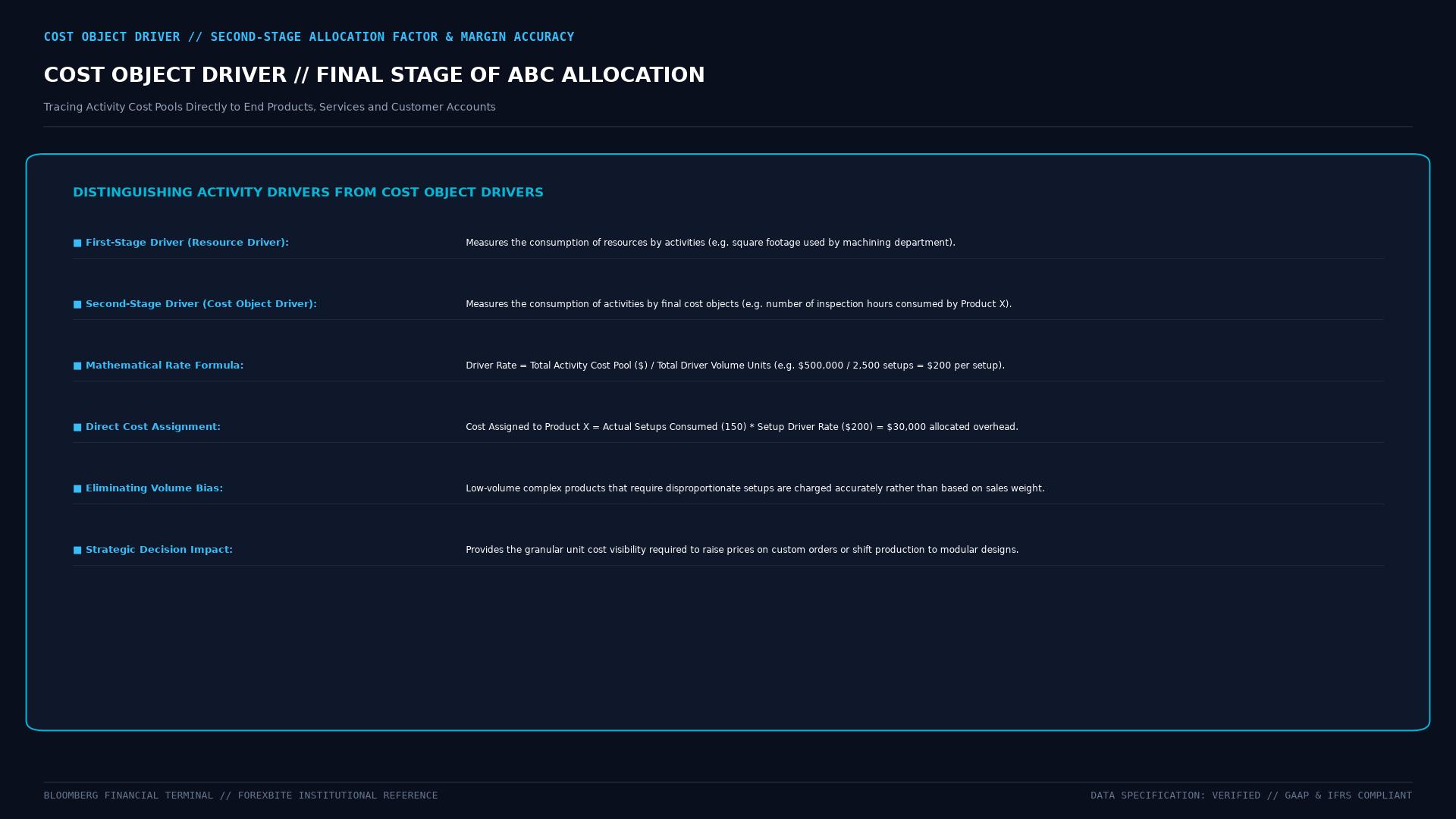 Figure: Operational mechanics of Cost-Object Drivers in assigning multi-activity costs to final products, customer segments, and service lines to prevent traditional volume-based margin distortions.
Architectural Role in the CAM-I Cross Framework
To understand the operational function of a cost object driver, examine the CAM-I Cost Management Cross model developed by leading international manufacturing accounting consortiums.
The CAM-I framework visualizes cost management as two intersecting axes:
- The Cost Assignment View (Vertical Axis): Tracks the downward flow of monetary resources through activities down to final cost objects. In this vertical axis, cost object drivers represent the final connection point, ensuring every dollar of corporate overhead is absorbed accurately based on actual operational consumption.
- The Process View (Horizontal Axis): Tracks the horizontal operational flow of business processes: Process Triggers $\rightarrow$ Activities $\rightarrow$ Performance Measures. Here, drivers provide the quantitative data needed to evaluate process cycle times, defect rates, and operational throughput.
+------------------------------------+------------------------------------+
| Stage 1: Resource Driver           | Stage 2: Cost Object Driver        |
+------------------------------------+------------------------------------+
| Assignment Target:                 | Assignment Target:                 |
| Links general ledger expense lines | Links intermediate activity cost   |
| to operational activity centers.   | pools to final billable products.  |
|                                    |                                    |
| Common Metrics:                    | Common Metrics:                    |
| Square footage, headcount ratios,  | Setup hours, machine runtime, bill |
| kilowatt hours, IT server cores.   | of materials line counts, calls.   |
|                                    |                                    |
| Primary Accounting Focus:          | Primary Accounting Focus:          |
| Cost accumulation within functional| Product pricing, margin analysis,  |
| operational departments.           | and customer profitability reviews.|
+------------------------------------+------------------------------------+
Mathematical Formulation of Cost Object Allocations
The mathematical mechanics of allocating intermediate activity pool costs to a final cost object involves two sequential calculations:
Step 1: Compute the Cost Object Driver Rate
The activity cost driver rate ($R_k$) is derived by dividing the total monetary expenses accumulated in activity pool $k$ by the practical capacity of the chosen driver ($D_k$):
$$R_k = \frac{\text{Total Activity Cost Pool}_k}{\text{Total Practical Capacity of Cost Object Driver}_k}$$
Step 2: Assign Costs to the Specific Cost Object
The overhead cost assigned to an individual cost object ($i$) from activity pool ($k$) equals the actual quantity of driver units consumed ($Q_{i,k}$) multiplied by the calculated rate:
$$\text{Assigned Activity Cost}{i,k} = Q{i,k} \times R_k$$
$$\text{Total Indirect Cost of Cost Object}i = \sum{k=1}^{M} (Q_{i,k} \times R_k)$$
Industrial Implementation Example
A contract biotechnology manufacturing laboratory operates an automated cell-culture bioreactor facility with an annual maintenance and clean-room sterilization activity cost pool of $3,600,000.
- Cost Object Driver Selected: Sterilization and Purge Hours ($D_k$).
- Total Practical Capacity: 1,200 sterilization hours per year.
- Cost Object Driver Rate ($R_k$): $\frac{$3,600,000}{1,200} = $3,000.00 \text{ per sterilization hour}$.
When evaluating two distinct pharmaceutical client contracts:
- Contract Alpha (Standard Monoclonal Antibody): High-volume production requiring only 4 sterilization hours per monthly batch. $$\text{Monthly Assigned Cost} = 4 \times $3,000 = $12,000$$
- Contract Beta (Customized Gene Therapy): Highly sensitive pathogen run requiring 25 sterilization and micro-filtration hours per batch due to contamination risks. $$\text{Monthly Assigned Cost} = 25 \times $3,000 = $75,000$$
Under traditional cost accounting that allocated facility overhead based on direct labor dollars or unit counts, Contract Alpha would have subsidized Contract Beta, masking the fact that Contract Beta was unprofitable at its agreed contract price.
Sector-Specific Cost Object Driver Applications
Cost object drivers vary across economic sectors depending on the complexity of the delivery model:
  Industry Sector      Intermediate Activity Pool       Selected Cost Object Driver
  ──────────────────────────────────────────────────────────────────────────
  Fintech & Banking    Payment Fraud Surveillance       Number of High-Risk API Queries
                       Wire Transfer Authentication     Count of Executed International Wires

  Healthcare           ICU Clinical Patient Care        Acuity-Adjusted Nursing Hours
                       Surgical Suite Sterilization     Operating Room Minutes per Procedure

  E-Commerce Logistics Hazardous Hazmat Packing         Specialized Handling Package Count
                       Long-Haul Fulfillment            Refrigerated Ton-Miles Transported

  Enterprise Software  Custom API Integration Support   Dedicated Senior Engineering Hours
                       Cloud Server Compute Provision   Virtual vCPU Hours Consumed per Tenant
Customer Profitability Analysis and the “Whale Curve”
A prominent application of cost object drivers in corporate strategy is Customer Profitability Analysis (CPA). When corporations treat individual client accounts as the final cost object, cost object drivers reveal stark truths about customer profitability.
In many enterprises, applying cost object drivers (such as number of expedited shipments, frequency of order change notices, specialized packaging requests, and post-sale technical support calls) generates the classic Whale Curve of Cumulative Profitability:
       THE WHALE CURVE OF CUMULATIVE CUSTOMER PROFITABILITY

  Cumulative Profit %
  200% │                                ┌──────────┐
       │                            ┌───┘          └────┐
  150% │                        ┌───┘                   └───┐
       │                    ┌───┘                           └───┐
  100% │                ┌───┘                                   └───┐ 100% Final Net
       │            ┌───┘                                           └───
   50% │        ┌───┘
       │    ┌───┘
    0% └────┴─────────────────────────────────────────────────────────── Customers
            20% "Peak" Customers       60% "Neutral"        20% "Loss" Customers
            (Yield 150%+ Profits)      (Break-Even)         (Destroy 50% Profit)
The top 20% of customers generate up to 150% of the enterprise true operating profit. The middle 60% generate break-even margins. The bottom 20% destroy 50% of total profits because their small order sizes and excessive customized demands trigger massive cost object driver charges.
Armed with accurate driver metrics, corporate executives can negotiate price increases, implement minimum order quantities, or terminate toxic accounts to restore overall corporate profitability.
Frequently Asked Questions
How does a company know if it has chosen the wrong cost object driver?
A company has chosen an inappropriate cost object driver if there is a weak statistical correlation ($R^2 < 0.60$) between the driver volume and total incurred activity costs, if tracking the driver requires expensive administrative time that exceeds the accuracy benefits, or if the driver metric creates perverse operational incentives (such as factory workers skipping safety checks to reduce measured setup time).
What is the difference between a cost object driver and a cost allocation base?
In traditional absorption costing, a cost allocation base is typically an arbitrary, company-wide volume metric (like total direct labor hours or direct materials cost) used to dump overhead onto products without proving causation. A cost object driver in Activity-Based Costing is specifically selected because it exhibits a demonstrable, verifiable cause-and-effect link between the cost object and the resource consumption of the activity.
Can an enterprise have too many cost object drivers?
Yes. Over-engineering an Activity-Based Costing system by creating hundreds of specialized cost object drivers creates high data-collection and software maintenance expenses, often leading to organizational abandonment of the ABC model. Modern managerial best practices favor Time-Driven Activity-Based Costing (TDABC), which consolidates multiple drivers into two standard variables: unit cost of capacity and time required to complete the activity.
Ready to trade forex?
Open a free demo account with a regulated broker. Practice with virtual funds before risking real money.