Autocorrelation

What is Autocorrelation in Financial Markets?

Autocorrelation—frequently termed serial correlation—measures the linear relationship between a time series variable and a lagged version of itself over sequential periods. In statistics, an independent variable is assumed to share zero correlation with its past values. In real-world currency and capital markets, however, price changes, trading volume, and volatility frequently exhibit non-random clusters and temporal linkages.

For quantitative analysts and algorithmic currency traders, autocorrelation serves as an empirical lens into market efficiency. If exchange rate returns display statistically significant autocorrelation, current returns contain predictive information regarding future price trajectories. Conversely, when autocorrelation hovers around zero, prices closely follow a random walk, invalidating simplistic predictive models.

---

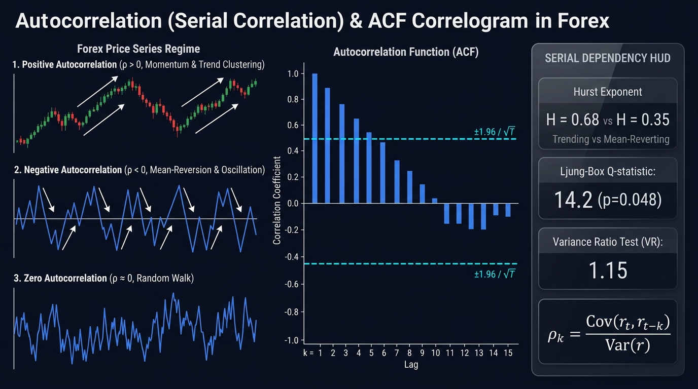
Mathematical Foundations: The Autocorrelation Function (ACF)

To calculate autocorrelation at a specific time lag $k$, analysts compute the covariance between current returns $r_t$ and lagged returns $r_{t-k}$, normalized by the variance of the series:

$$\rho_k = \frac{\sum_{t=k+1}^T (r_t - \bar{r})(r_{t-k} - \bar{r})}{\sum_{t=1}^T (r_t - \bar{r})^2}$$

Where:

• $\rho_k$ = Autocorrelation coefficient at lag $k$ (bounded between $-1$ and $+1$).
• $r_t$ = Asset return at time period $t$.
• $r_{t-k}$ = Asset return $k$ periods prior.
• $\bar{r}$ = Mean return across the entire sample period $T$.

Plotting $\rho_k$ across various lags ($k = 1, 2, 3, \dots, 20$) yields an Autocorrelation Function (ACF) plot, commonly known as a correlogram.

---

Interpreting Serial Correlation Regimes

The magnitude and algebraic sign of the autocorrelation coefficient provide distinct behavioral insights into underlying market microstructure:

1. Positive Autocorrelation ($\rho > 0$)

• Market Dynamic: Momentum and trend persistence.
• Behavioral Driver: Institutional capital taking hours or days to execute large block orders, cascading algorithmic stops, or slow assimilation of macroeconomic news.
• Trading Implication: Favors trend-following strategies, breakout systems, and moving average cross algorithms.

2. Negative Autocorrelation ($\rho < 0$)

• Market Dynamic: Anti-persistence, mean-reversion, and oscillation.
• Behavioral Driver: Market-maker inventory balancing, the bid-ask bounce effect (trades alternating between the bid and ask), and liquidity exhaustion at key support and resistance zones.
• Trading Implication: Favors statistical arbitrage, range-trading strategies, and mean-reverting Bollinger Band oscillators.

3. Zero Autocorrelation ($\rho \approx 0$)

• Market Dynamic: White noise and weak-form market efficiency.
• Behavioral Driver: Instantaneous assimilation of public information by deep market liquidity.
• Trading Implication: Linear forecasting models fail; traders must rely on non-linear dynamics, order flow imbalances, or volatility trading.

---

Practical Trading Example: Microstructure vs. Macro Lags on GBP/USD

Consider a quantitative hedge fund assessing serial correlation on the GBP/USD currency pair across two distinct time resolutions:

Case A: 1-Second Tick Data (High-Frequency Order Flow)

Running an ACF analysis on raw 1-second price changes reveals:

• Lag 1 ($\rho_1$): $-0.32$ (Statistically significant negative correlation).
• Diagnosis: The negative lag-1 autocorrelation is an artifact of the bid-ask bounce. Trades are sequentially crossing between the dealer bid (1.2700) and the dealer ask (1.2701).
• Strategy Implementation: The algorithm does not enter momentum breakout trades at this scale; instead, it provides passive liquidity as a market maker to harvest the spread.

Case B: 1-Day Log Returns (Macroeconomic Post-Announcement Drift)

Running an ACF analysis on daily returns during central bank tightening cycles reveals:

• Lag 1 ($\rho_1$): $+0.18$ (Statistically significant positive correlation).
• Lag 2 ($\rho_2$): $+0.12$.
• Diagnosis: Interest rate divergences create multi-day trending persistence as institutional pension funds reallocate global asset weightings over several trading sessions.
• Strategy Implementation: The model activates a systematic trend-following overlay, holding long positions following positive daily closing momentum.

---

Quantitative Diagnostic Tests

Traders validate whether observed autocorrelation represents true structural signal rather than random sampling noise using formal econometric tests:

Statistical Test	Primary Purpose	Test Metric / Threshold	Practical Application
Durbin-Watson Test ($d$)	Tests for first-order serial correlation ($\rho_1$) in regression residuals.	Scales from 0 to 4 ($d \approx 2$ indicates zero autocorrelation; $d < 2$ indicates positive; $d > 2$ indicates negative).	Validates algorithmic regression models to ensure residuals are not carrying trend bias.
Ljung-Box Q-Test	Evaluates whether a group of autocorrelations across multiple lags ($k$) is simultaneously non-zero.	$p$-value $< 0.05$ rejects the null hypothesis of independence.	Determines whether an entire time series possesses exploitable memory or behaves as white noise.
Variance Ratio Test	Compares return variance across multiple holding periods against the linear scaling rule of random walks.	Variance ratio $\neq 1.0$ indicates serial dependency.	Differentiates long-term drift from temporary cyclical regimes.

---

Pitfalls: Non-Stationarity and Volatility Clustering

1. The Spurious Correlation Trap (Raw Prices vs. Log Returns): Evaluating autocorrelation on raw currency exchange rates (e.g., EUR/USD spot levels) will virtually always show an autocorrelation coefficient near $+0.99$. This is a mathematical illusion caused by non-stationarity—the series wanders over time. Valid analysis requires first-differencing the series into percentage or log returns: $r_t = \ln(P_t / P_{t-1})$.

2. Volatility Clustering (ARCH Effect): While linear price returns in liquid currency pairs often show zero autocorrelation, the squared returns ($r_t^2$) or absolute returns ($|r_t|$) routinely display massive positive autocorrelation. Large price swings—regardless of direction—are followed by large price swings, forming the basis for GARCH volatility modeling.

---

Comparative Matrix: Autocorrelation Across Timeframes

Timeframe	Typical Autocorrelation Sign	Primary Cause	Dominant Trading Style
Sub-Second / Tick	Strongly Negative ($\rho < -0.25$)	Bid-Ask Bounce, order matching queue	High-Frequency Market Making
1-Minute to 15-Minute	Weakly Negative or Zero	Order book absorption, algorithmic rebalancing	Mean Reversion / Scalping
4-Hour to Daily	Moderately Positive ($\rho > +0.10$)	Trend continuation, institutional execution	Swing Trading, Breakout Trading
Monthly / Quarterly	Weakly Negative / Mean Reverting	Macroeconomic valuation cycles, PPP adjustments	Value Investing, Carry Trade Unwinding

---

Key Takeaways

• Autocorrelation measures the statistical correlation between an asset’s past and future price returns across specified time lags.
• A positive autocorrelation indicates momentum persistence, where positive periods are followed by positive periods.
• A negative autocorrelation indicates anti-persistence or mean-reversion, characteristic of market microstructure noise and range-bound environments.
• Raw price series must be converted to stationary returns to prevent spurious, deceptive correlation readings.
• While linear returns often appear unpredictable on intermediate timeframes, squared returns exhibit strong volatility clustering, proving that volatility itself is highly autocorrelated.

---

Frequently Asked Questions

What does negative autocorrelation mean in forex trading?

Negative autocorrelation means that a positive price move in one period is statistically more likely to be followed by a negative price move in the next period, and vice versa. It signals a mean-reverting or oscillating environment, making trend-following strategies unprofitable and favoring range-bound scalping.

What is the difference between autocorrelation and standard correlation?

Standard correlation compares two distinct variables (such as the relationship between EUR/USD and Gold). Autocorrelation measures the internal relationship within a single variable across successive time periods (such as how EUR/USD today correlates with EUR/USD yesterday).

Why do daily currency returns show low linear autocorrelation?

According to the Efficient Market Hypothesis, liquid financial assets quickly incorporate all accessible information into prices. If daily returns were reliably autocorrelated, arbitrageurs would exploit the pattern until price adjustments eliminated the predictive signal.

How does the Durbin-Watson statistic detect autocorrelation?

The Durbin-Watson test produces a test statistic ranging from 0 to 4. A value near 2.0 indicates no serial correlation in regression residuals. Values substantially below 2.0 signal positive serial correlation, while values approaching 4.0 signal negative serial correlation.