Factor Analysis
A multivariate statistical method used to explain the variance and covariance among a large set of observed financial variables through a lower number of unobserved latent factors, serving as the core engine for quantitative asset pricing and risk modeling.
Factor Analysis
Factor analysis is a multivariate statistical framework designed to describe the variability and covariances among a large collection of observed, correlated assets in terms of a significantly smaller number of unobserved, latent variables known as factors. Instead of treating every individual equity, currency pair, or corporate bond as an independent price series, factor analysis identifies the common underlying economic forces that cause thousands of securities to fluctuate in harmony.
In modern quantitative asset management, hedge fund risk budgeting, and algorithmic execution, factor analysis forms the mathematical engine behind systematic investing. Whether applied through exploratory statistical extraction (such as Principal Component Analysis) or structured economic models (such as the Fama-French multi-factor frameworks and MSCI Barra risk models), factor decomposition allows quantitative analysts to strip away idiosyncratic market noise, isolate systematic market drivers, and engineer portfolios with targeted risk exposures.
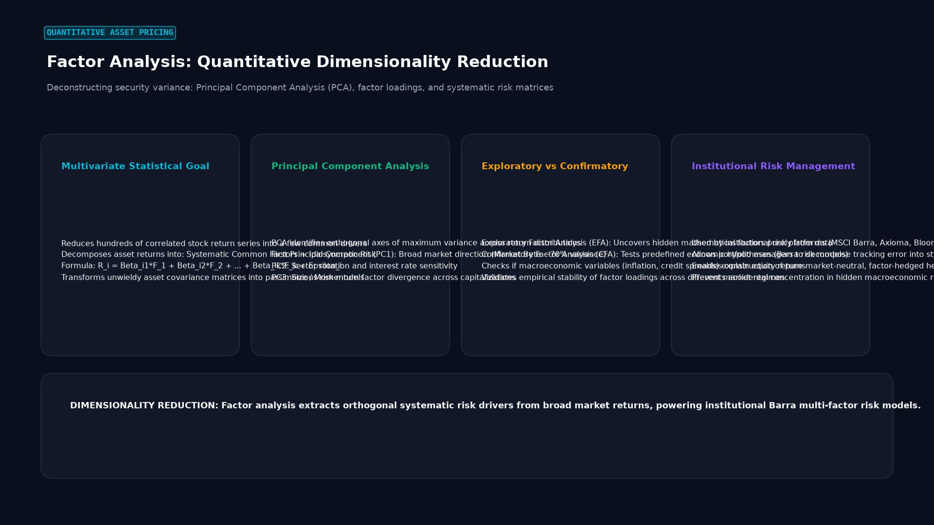 Figure: Deconstructing security variance: Principal Component Analysis (PCA), factor loadings, and systematic risk matrices
Mathematical Formulation and Matrix Mechanics
The classical linear factor model expresses the vector of $N$ observed asset returns at time $t$ as a linear combination of $K$ unobserved common factors, plus an asset-specific idiosyncratic error term ($K \ll N$):
$$R_{it} - R_{ft} = \alpha_i + \lambda_{i1} F_{1t} + \lambda_{i2} F_{2t} + \dots + \lambda_{iK} F_{Kt} + \epsilon_{it}$$
In matrix notation across all $N$ assets, the system is expressed as:
$$\mathbf{R}_t = \boldsymbol{\alpha} + \boldsymbol{\Lambda} \mathbf{F}_t + \boldsymbol{\epsilon}_t$$
Where:
- $\mathbf{R}_t$ is an $N \times 1$ vector of observed asset excess returns over the risk-free rate $R_f$.
- $\boldsymbol{\alpha}$ is an $N \times 1$ vector of intercepts representing unexplained excess returns (alpha).
- $\boldsymbol{\Lambda}$ is an $N \times K$ matrix of factor loadings (often referred to as factor betas or exposures), where element $\lambda_{ik}$ represents the sensitivity of asset $i$ to changes in factor $k$.
- $\mathbf{F}_t$ is a $K \times 1$ vector of realized common factor returns at time $t$.
- $\boldsymbol{\epsilon}_t$ is an $N \times 1$ vector of idiosyncratic error terms (specific risk), assumed to have zero mean ($\mathbb{E}[\boldsymbol{\epsilon}_t] = \mathbf{0}$) and to be uncorrelated with the common factors ($\text{Cov}(\mathbf{F}_t, \boldsymbol{\epsilon}_t) = \mathbf{0}$).
+--------------------------------------------------------------------------+
|                  Covariance Matrix Decomposition Engine                  |
+--------------------------------------------------------------------------+
|                                                                          |
|  The total N x N covariance matrix of asset returns (Σ) decomposes as:   |
|                                                                          |
|                     Σ = Λ * Φ * Λ' + Ψ                                   |
|                                                                          |
|  Where:                                                                  |
|  - Σ is the N x N empirical covariance matrix of asset returns.          |
|  - Λ is the N x K matrix of factor loadings (systematic sensitivities).  |
|  - Φ is the K x K covariance matrix of the common factors.              |
|  - Ψ is an N x N diagonal matrix of unique, asset-specific variances:    |
|         Ψ = diag(σ^2_{ε_1}, σ^2_{ε_2}, ..., σ^2_{ε_N})                   |
|                                                                          |
+--------------------------------------------------------------------------+
Communality and Uniqueness
For any individual asset $i$, its total variance $\sigma_i^2$ is partitioned into two distinct components:
$$\sigma_i^2 = h_i^2 + \psi_i$$
- Communality ($h_i^2$): The proportion of the asset’s total variance explained by the common systematic factors ($h_i^2 = \sum_{k=1}^K \lambda_{ik}^2 \text{Var}(F_k)$). Assets with high communality (such as large-cap banking stocks) move in lockstep with broad macroeconomic and market factors.
- Uniqueness or Specific Variance ($\psi_i$): The residual proportion of variance attributable strictly to company-specific events (e.g., patent litigation, internal management restructuring). This specific risk is diversifiable in a broad portfolio.
Factor Extraction Methodologies
Quantitative analysts utilize three primary extraction techniques to identify common factors from historical return series:
+--------------------------------------------------------------------------+
|                  Comparison of Factor Extraction Techniques              |
+--------------------------------------------------------------------------+
|  Methodology          | Mathematical Mechanism  | Financial Application  |
+-----------------------+-------------------------+------------------------+
|  Principal Component  | Spectral decomposition  | Unsupervised data      |
|  Analysis (PCA)       | of sample covariance /  | reduction; exploratory |
|                       | correlation matrix      | yield curve modeling   |
|  Maximum Likelihood   | Iterative parameter     | Confirmatory hypothesis|
|  Estimation (MLE)     | estimation assuming     | testing; academic risk |
|                       | multivariate normality  | factor validation      |
|  Independent Component| Higher-order cumulant   | Non-linear tail risk;  |
|  Analysis (ICA)       | maximization (kurtosis) | flash crash and regime |
|                       | separating non-Gaussian | shift detection        |
+--------------------------------------------------------------------------+
1. Principal Component Analysis (PCA)
PCA constructs orthogonal linear combinations of original asset returns that maximize explained variance:
- The first principal component ($PC_1$) captures the direction of greatest variance across the asset universe (in equities, this invariably corresponds to the broad market direction).
- The second principal component ($PC_2$) captures the maximum remaining variance orthogonal (uncorrelated) to $PC_1$.
In fixed-income markets, applying PCA to sovereign yield curve tenors famously extracts three dominant components that explain over 98% of all yield curve movements: Level (parallel shifts), Slope (steepening or flattening), and Curvature (butterfly shifts).
2. Maximum Likelihood Factor Analysis
Unlike PCA, which focuses purely on total variance maximization, maximum likelihood factor analysis explicitly models the distinction between common variance and unique variance ($\psi_i$). By assuming that asset returns follow a multivariate normal distribution, MLE iteratively solves for the factor loading matrix $\boldsymbol{\Lambda}$ and the specific variance matrix $\boldsymbol{\Psi}$ that maximize the probability of observing the empirical sample covariance matrix.
Factor Rotation and Economic Interpretability
Raw mathematical factors extracted via PCA or MLE are purely statistical constructs. They maximize variance mathematically, but individual factors often feature messy cross-loadings that lack clear economic meaning.
To transform statistical abstractions into actionable investment themes, analysts apply factor rotation:
                 Orthogonal Varimax Rotation of Factor Axes
  Factor 2 (Growth Loading)
      ^
      |           * Tech Stock A
      |          /
      |         /  Rotated Axis 2
      |        /
      |       /   * Tech Stock B
      |      /
      |     /                   Rotated Axis 1
      |    /              . . . . . . . . . . . . . . * Bank Stock C
      |   /       . . . *
      |  / . . . *
      +---------------------------------------------------------->
0 Factor 1 (Value Loading)- Orthogonal Rotation (Varimax): Keeps factor axes strictly perpendicular (uncorrelated at 90 degrees). Varimax maximizes the variance of squared loadings across variables, driving loadings to either near 1.0 or near 0.0. This isolates pure, independent factor bets (e.g., pure Value vs. pure Momentum).
- Oblique Rotation (Promax): Relaxes the requirement that factors remain uncorrelated. In real-world capital markets, economic drivers frequently correlate during systemic crises (for example, small-cap stocks frequently exhibit high cyclical beta). Promax rotation provides superior empirical fit during stress periods by permitting realistic correlations between factor axes.
Multi-Factor Asset Pricing Models in Practice
Factor analysis underpins the progression of asset pricing theory from single-index models to multi-dimensional risk engines:
+--------------------------------------------------------------------------+
|                  The Evolution of Factor Pricing Architectures           |
+--------------------------------------------------------------------------+
|                                                                          |
|  [ 1964: Sharpe-Lintner CAPM ] ───► Single Factor: Market Beta (MKT)     |
|                                                                          |
|  [ 1976: Ross Arbitrage Pricing ] ──► Generalized Multi-Factor (APT)     |
|                                                                          |
|  [ 1993: Fama-French 3-Factor ] ──► Market + Size (SMB) + Value (HML)    |
|                                                                          |
|  [ 1997: Carhart 4-Factor ] ──────► Fama-French 3 + Momentum (WML)       |
|                                                                          |
|  [ 2015: Fama-French 5-Factor ] ──► Adds Profitability (RMW) + Inv (CMA) |
|                                                                          |
+--------------------------------------------------------------------------+
The Fama-French 5-Factor Model
Eugene Fama and Kenneth French proved that single-factor CAPM beta failed to explain the cross-section of expected equity returns. Their expanded model evaluates five structural factors:
$$R_{it} - R_{ft} = \alpha_i + \beta_{i1} \text{MKT}t + \beta{i2} \text{SMB}t + \beta{i3} \text{HML}t + \beta{i4} \text{RMW}t + \beta{i5} \text{CMA}t + \epsilon{it}$$
Where:
- $\text{MKT}_t$ is the market excess return.
- $\text{SMB}_t$ (Small Minus Big) measures the historical return premium of small-cap stocks over large-cap stocks.
- $\text{HML}_t$ (High Minus Low) measures the value premium of high book-to-market equities over low book-to-market growth equities.
- $\text{RMW}_t$ (Robust Minus Weak) captures the premium of companies with robust operating profitability over weak profitability.
- $\text{CMA}_t$ (Conservative Minus Aggressive) measures the excess return of firms that invest conservatively over those that expand assets aggressively.
Portfolio Construction and Risk Factor Budgeting
Modern quantitative asset allocators do not allocate capital across asset classes (equities, bonds, real estate). Instead, they allocate across underlying risk factors:
[ Institutional Asset Universe: 3,000 Global Equities & Debt Issues ]
                                │
                                ▼
[ Ingest Return History & Balance Sheet Descriptors ]
                                │
                                ▼
[ Run Cross-Sectional Factor Regression / Covariance Decomposition ]
                                │
                                ▼
[ Map Portfolio Holdings to Fundamental Risk Factors ]
  - Equity Market Beta: 0.85
  - Duration Risk: 4.2 Years
  - Credit Spread Risk (CSWAP): 120 bps
  - FX Momentum Loading: +0.42
                                │
                                ▼
[ Optimize Factor Balance: Risk Parity Allocation Across Factors ]
Risk Parity Across Factors
In a traditional 60/40 equity-bond portfolio, equity risk accounts for more than 90% of total portfolio volatility because equity market variance dwarfs fixed-income variance. By applying factor analysis, quantitative managers equalize the marginal contribution to risk (MCR) of each latent factor:
$$\text{MCR}_k = \frac{\partial \sigma_p}{\partial w_k} = \frac{(\boldsymbol{\Lambda} \boldsymbol{\Phi})_k}{\sigma_p}$$
Leveraging low-volatility factors (such as short-dated sovereign duration) while scaling back high-beta equity exposure produces a resilient portfolio that delivers steady risk-adjusted returns across deflationary and inflationary regimes.
Case Study: Cross-Asset Contagion in March 2020
During the onset of the COVID-19 pandemic in March 2020, institutional multi-asset funds experienced catastrophic correlation breakdowns:
- Traditional diversification failed: US equities, corporate investment-grade bonds, emerging market debt, and physical gold all sold off simultaneously.
- Standard risk models projected that gold and Treasuries would rally to offset equity drawdowns. Instead, margin calls forced multi-strategy hedge funds to liquidate liquid safe-haven assets.
+--------------------------------------------------------------------------+
|                  March 2020 Factor Decomposition Findings                |
+--------------------------------------------------------------------------+
|  Historical Factor Mix   | Explains 85% of returns during calm regimes   |
|  March 2020 Spike        | Single "US Dollar Liquidity" Factor surged,   |
|                          | explaining over 70% of cross-asset variance   |
|  Unhedged Funds          | Sustained 15% to 25% portfolio drawdowns      |
|  Factor-Hedged Desks     | Pre-hedged dollar liquidity via FX swaps and  |
|                          | short index futures, capping losses at <4%    |
+--------------------------------------------------------------------------+
Factor analysis conducted by institutional risk platforms (including BlackRock’s Aladdin) revealed that cross-asset returns were dominated by a single latent variable: acute US dollar funding liquidity. Desks that monitored their factor loading on USD liquidity were able to purchase offshore currency swaps and VIX options, immunizing their balance sheets before central banks initiated emergency swap facilities.
Methodological Traps and Econometric Hazards
Quantitative analysts must navigate several severe statistical traps when deploying factor analysis:
- Look-Ahead and In-Sample Overfitting: Extracting factors over a full historical backtest window introduces look-ahead bias. True quantitative models must utilize expanding rolling windows or out-of-sample testing to ensure factor loadings were identifiable in real time.
- Factor Zoo Proliferation: Academic finance has published over 400 distinct “factors” claiming to predict stock returns. Most of these anomalies are the product of multiple testing bias (p-hacking). Analysts apply Bonferroni adjustments or the Harvey-Liu-Zhu hurdle rate (mandating a t-statistic of $t \ge 3.0$) before acknowledging a newly proposed factor.
- Regime Instability and Non-Stationarity: Factor loadings are not static physical constants. A company’s sensitivity to interest rate duration or energy prices shifts dramatically as corporate debt matures or business lines evolve. Static factor models break down during macro inflection points.
Frequently Asked Questions
What is the difference between factor analysis and Principal Component Analysis?
PCA is a data reduction technique that transforms observed variables into orthogonal linear combinations to explain total variance, without distinguishing between common variance and asset-specific error. Factor analysis assumes a formal underlying statistical model, separating common variance shared across assets from idiosyncratic, asset-specific unique variance.
How do analysts determine how many factors to retain?
Analysts employ three primary criteria: the Kaiser criterion (retaining factors with eigenvalues greater than 1.0), the Scree plot elbow test (identifying the graphical point where the downward slope of eigenvalues flattens), and parallel analysis (comparing empirical eigenvalues against eigenvalues generated from randomized synthetic data).
Can factor analysis capture non-linear market shocks?
Standard linear factor analysis struggles to capture non-linear tail events, asymmetric volatility, and sudden regime shifts. To model non-linear phenomena, quantitative researchers utilize Kernel Factor Analysis, Independent Component Analysis (ICA), or deep learning autoencoder architectures that extract non-linear latent manifolds from return series.
Ready to trade forex?
Open a free demo account with a regulated broker. Practice with virtual funds before risking real money.