Value at Risk (VaR) — Forex Dictionary Definition

What Is Value at Risk (VaR)?

Value at Risk (VaR) is the institutional gold standard for summarizing and communicating market risk across multi-asset trading desks, banks, and investment funds. By synthesizing diverse financial exposures—including spot foreign exchange, equity options, corporate debt, and commodities—into a single currency figure, VaR answers a vital executive question: “What is the maximum amount we stand to lose over horizon $T$ with $(1 - \alpha)%$ confidence?”

For example, if an institutional foreign exchange trading desk reports a 1-day $99%$ VaR of $$5\text{ million}$, it implies that under normal market operating conditions, there is a $99%$ statistical probability that the desk’s daily loss will not exceed $$5\text{ million}$. Conversely, there is a $1%$ chance (occurring on average about $2.5$ trading days per year) that daily losses will exceed that $$5\text{ million}$ threshold.

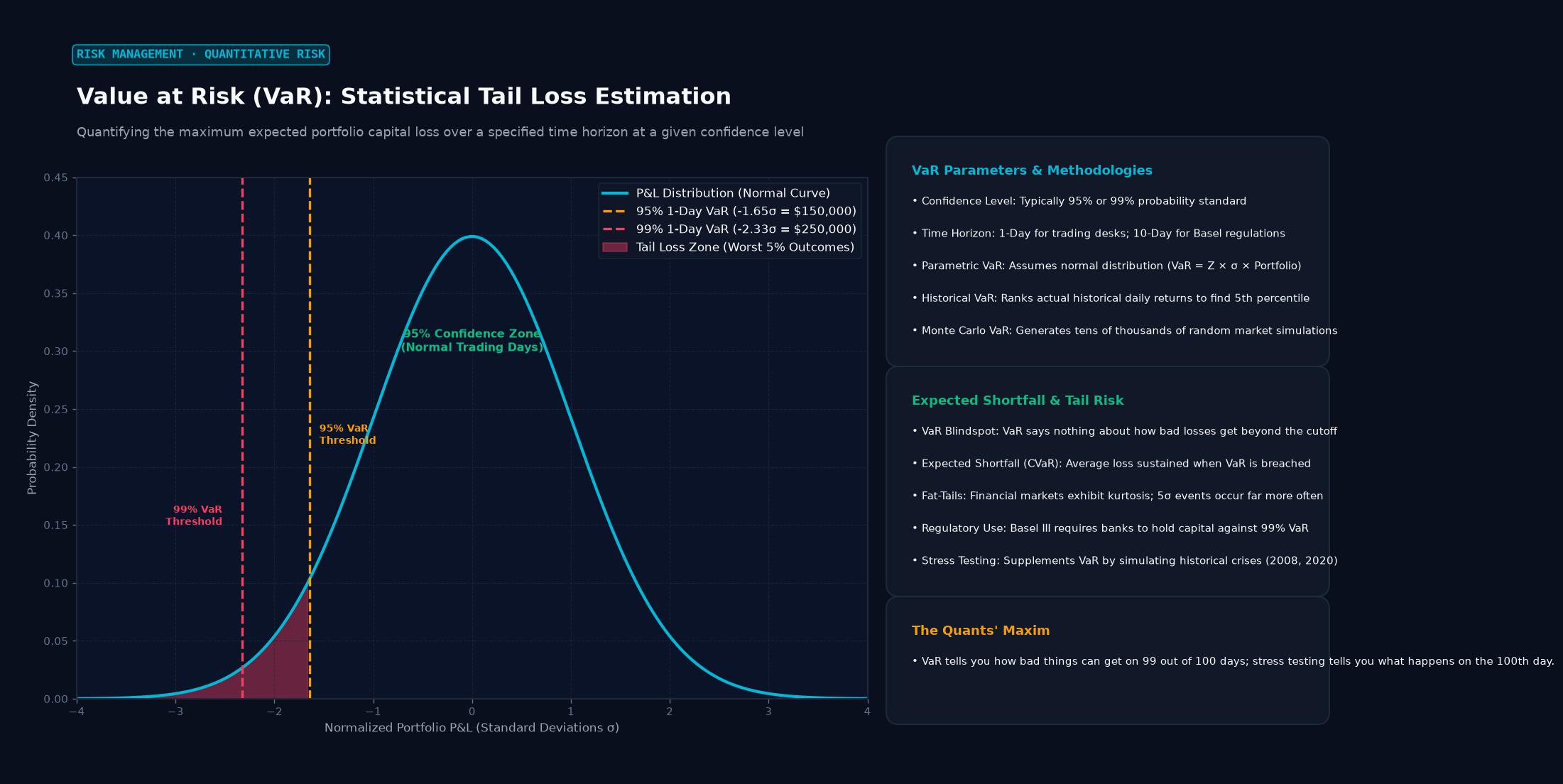Value at Risk (VaR): Statistical Tail Loss Estimation Figure: Quantifying the maximum expected portfolio capital loss over a specified time horizon at a given confidence level

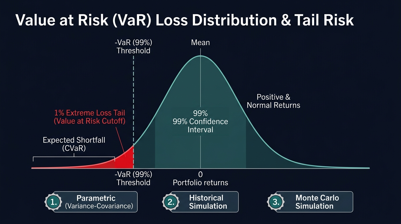
Value at Risk (VaR) Loss Distribution and Tail Risk Diagram

Mathematical Formulation: The Three Methodologies

Formally, given a cumulative loss distribution function $F_L(l) = P(L \le l)$, the Value at Risk at confidence level $\alpha \in (0, 1)$ is the $(1 - \alpha)$-quantile:

$$\text{VaR}_{\alpha} = \inf { l \in \mathbb{R} : P(L > l) \le 1 - \alpha }$$

Quantitative risk management computes VaR using three primary modeling frameworks:

1. Parametric (Variance-Covariance) VaR

Assumes portfolio asset returns follow an elliptical multivariate normal distribution. For a linear portfolio of value $\Pi$ with aggregate volatility $\sigma_p$ over time horizon $\Delta t$:

$$\text{VaR}{\alpha, \Delta t} = \Pi \times Z{\alpha} \times \sigma_p \times \sqrt{\Delta t}$$

Where $Z_{\alpha}$ is the standard normal inverse cumulative distribution value ($Z_{0.95} = 1.645$, $Z_{0.99} = 2.326$).

2. Historical Simulation VaR

Applies actual historical daily market price shifts (typically over the preceding 500 to 1,000 trading days) to the current portfolio book without making parametric distribution assumptions, capturing empirical skewness and kurtosis.

3. Monte Carlo Simulation VaR

Generates tens of thousands of pseudo-random market price paths using stochastic differential equations (e.g., Geometric Brownian Motion or Heston stochastic volatility models), enabling non-linear repricing of complex exotic options and structured notes.

Beyond VaR: Expected Shortfall (CVaR)

A fundamental theoretical flaw in standard VaR is that it does not satisfy the subadditivity axiom of coherent risk measures ($\text{VaR}(A+B) > \text{VaR}(A) + \text{VaR}(B)$ can occur under fat-tailed distributions). Furthermore, VaR is blind to the severity of losses beyond the confidence threshold.

To resolve this blind spot, the Basel Committee on Banking Supervision transitioned regulatory capital requirements (under Basel III / Fundamental Review of the Trading Book - FRTB) to Expected Shortfall (ES), also known as Conditional VaR (CVaR):

$$\text{ES}{\alpha} = \mathbb{E}[L \mid L > \text{VaR}{\alpha}]$$

While VaR answers “How bad could things get with $99%$ confidence?”, Expected Shortfall answers “If the $1%$ catastrophic tail event occurs, what is our expected average loss?”

VaR Frameworks Compared

Methodology	Computational Speed	Non-Linear Instrument Handling	Fat-Tail Accuracy	Model Risk / Vulnerability
Parametric (Normal)	Real-time (Milliseconds)	Poor (Linear delta approximation only)	Extremely Poor (severely underestimates fat tails)	Fails during market panics and volatility spikes
Historical Simulation	Fast to Moderate	Good (Full repricing possible)	Realistic based on past sample	Backward-looking; cannot simulate unprecedented shocks
Monte Carlo	High computational cost	Exceptional (Prices multi-asset path-dependent exotics)	Flexible (Can incorporate jump-diffusion and Student’s t)	Parameter misspecification; random number generator noise
Expected Shortfall (ES)	Moderate to High	High (Captures average tail density)	Superior (Subadditive coherent risk metric)	Requires dense tail sampling; backtesting complexity

Real-World Institutional Case Study: J.P. Morgan’s RiskMetrics & The LTCM 1998 Breakdown

The global adoption of VaR originated in 1989 when J.P. Morgan CEO Dennis Weatherstone demanded a standardized report delivered to his desk every afternoon at 4:15 PM summarizing the bank’s entire global market risk on a single page. J.P. Morgan’s quantitative research team formulated the RiskMetrics system, making the mathematical architecture public in 1994 and standardizing VaR across Wall Street.

However, the catastrophic vulnerability of parametric VaR was exposed in August 1998 by the collapse of Long-Term Capital Management (LTCM):

[LTCM Quantitative Model Predication]
Fund held $125 Billion in balance sheet assets and $1.25 Trillion in derivatives
Parametric VaR assumed normal distributions and historical cross-market correlations
Risk model projected maximum daily loss should not exceed $35 Million (a 3-sigma event)

[August 17, 1998: Russian Sovereign Debt Default]
Global liquidity evaporated; correlations across non-Russian sovereign debt jumped to 1.0
                    |
                    v
ACTUAL EXPERIENCE: LTCM lost $553 Million in a single day (A theoretical "10-Sigma Event")
Loss was mathematically impossible under their Gaussian VaR model
                    |
                    v
Fund lost 90% of its capital in 6 weeks; Federal Reserve Bank of New York
forced to coordinate a $3.65 Billion emergency Wall Street consortium bailout

The LTCM disaster proved that calculating VaR under normal distribution assumptions in highly leveraged portfolios creates a dangerous illusion of safety, leading modern quantitative desks to supplement VaR with rigorous stress testing and historical scenario analyses (e.g., simulating 1987 Black Monday, 2008 Lehman, or 2020 COVID).

Frequently Asked Questions

What does “1-day 95% VaR of $100,000” mean?

It means there is a $95%$ probability that the portfolio will not lose more than $$100,000$ over the next 24-hour trading session. Put another way, on 1 trading day out of every 20 ($5%$ of trading days), the portfolio is expected to experience losses exceeding $$100,000$.

Why did the Basel Committee replace VaR with Expected Shortfall?

The Basel Committee replaced $99%$ VaR with $97.5%$ Expected Shortfall because standard VaR completely ignores the magnitude of tail risk. Two portfolios can have identical $$1\text{ million}$ VaR figures, yet one portfolio might lose $$1.1\text{ million}$ in the tail while the other loses $$50\text{ million}$ due to hidden short option gamma risk. Expected Shortfall captures and penalizes this severe tail convexity.

How does market liquidity affect Value at Risk calculations?

Standard VaR assumes positions can be liquidated instantly at prevailing market prices. In illiquid markets (such as emerging market currencies or distressed corporate debt), liquidating a large position requires days or weeks, incurring severe market impact costs. Risk managers adjust for this by calculating Liquidity-Adjusted VaR (L-VaR), scaling the holding period horizon ($T$) to reflect the asset’s true liquidation half-life.