Factor Return

What Is a Factor Return?

In quantitative finance, empirical asset pricing, and institutional performance attribution, a factor return represents the portion of an investment’s return that is directly attributable to its exposure to a pervasive, systematic driver of risk.

Financial assets do not generate returns in isolation; their performance is determined by how sensitive they are to macroeconomic and style factors—such as broad market movements, credit spreads, value vs. growth valuation spreads, momentum trends, and size characteristics. The factor return is the specific price or payoff that the market awards to investors for bearing one unit of that factor’s risk over a specified period.

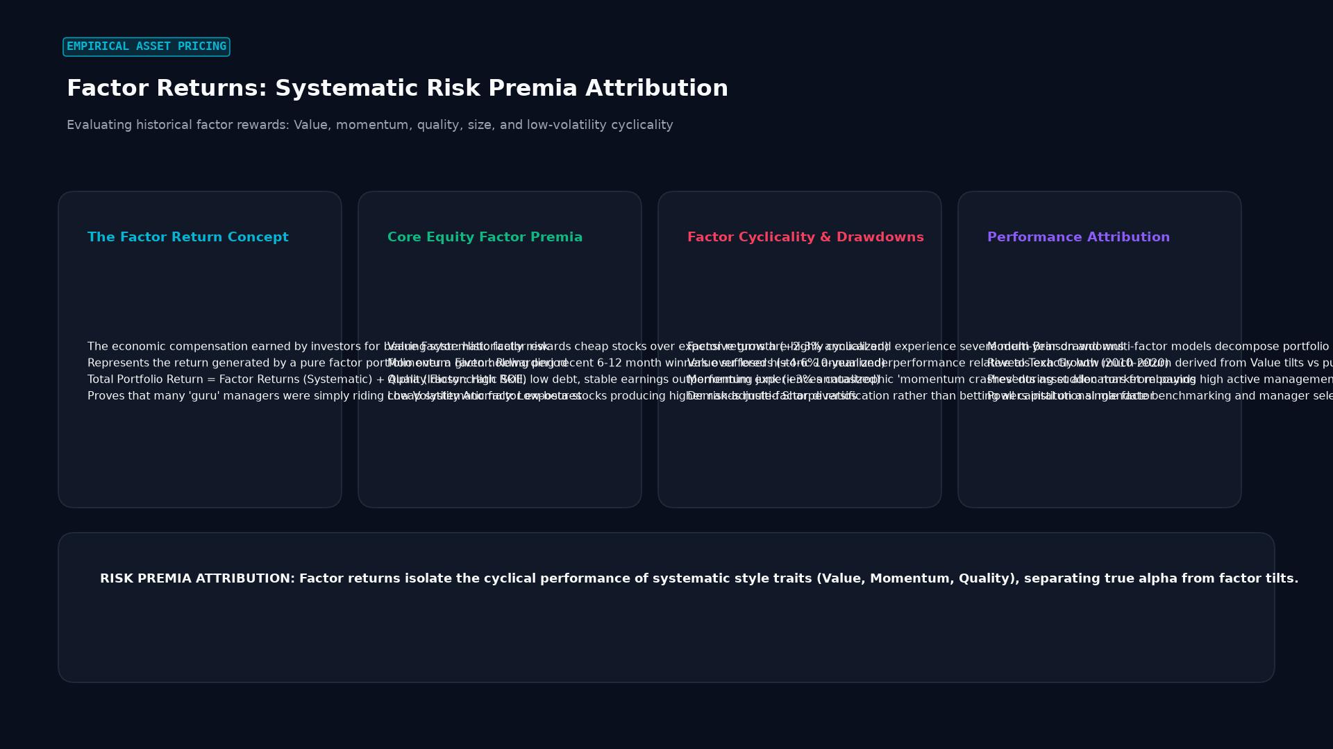Figure: Evaluating historical factor rewards: Value, momentum, quality, size, and low-volatility cyclicality

---

Technical Mechanics & Estimation Methodologies

Institutional risk engines (e.g., MSCI Barra, Axioma, Bloomberg PORT) estimate factor returns across universes using two primary mathematical methodologies:

1. The Fama-MacBeth Cross-Sectional Regression

The gold standard for estimating factor returns across cross-sectional panels is the two-pass regression methodology developed by Eugene Fama and James MacBeth (1973):

Step 1 (Time-Series): Estimate factor exposures ($\beta_{i,k}$) for each individual asset $i$ over historical rolling windows:

$$R_{i,t} - R_{f,t} = \alpha_i + \sum_{k=1}^K \beta_{i,k} F_{k,t} + \varepsilon_{i,t}$$

Step 2 (Cross-Sectional): At each time point $t$, run a cross-sectional regression of asset excess returns on their estimated factor betas to determine the realized factor return $\lambda_{k,t}$:

$$R_{i,t} = \lambda_{0,t} + \sum_{k=1}^K \beta_{i,k} \lambda_{k,t} + \eta_{i,t}$$

Where $\lambda_{k,t}$ represents the realized factor return for factor $k$ at time $t$. The long-run expected factor premium is the time-series average:

$$\bar{\lambda}k = \frac{1}{T} \sum{t=1}^T \lambda_{k,t}$$

2. Weighted Least Squares (WLS) Factor Extraction

Because asset residuals exhibit heteroskedasticity and market-cap disparities, commercial risk models employ Weighted Least Squares (WLS) or Generalized Least Squares (GLS) using the square root of market capitalization as regression weights:

$$f_t = \left( X^T W X \right)^{-1} X^T W R_t$$

Where:

• $X \in \mathbb{R}^{N \times K}$ is the standardized factor exposure matrix at time $t$.
• $W \in \mathbb{R}^{N \times N}$ is the diagonal weight matrix.
• $R_t \in \mathbb{R}^N$ is the vector of asset returns.
• $f_t \in \mathbb{R}^K$ is the estimated vector of factor returns.

---

Comparative Matrix: Return Classifications

Metric / Term	Driver of Return	Systematically Compensated?	Estimator	Key Risk Component
Factor Return	Common systematic risk factor (Value, Size, Yield)	Yes (positive long-term risk premium)	Cross-sectional regression / pure factor portfolio	Systematic market risk
Asset Return	Total combined price change and dividends	Yes (aggregate total)	Direct observation ($P_t / P_{t-1} - 1$)	Total risk (systematic + idiosyncratic)
Alpha ($\alpha$)	Idiosyncratic manager skill / structural mispricing	No (zero-sum market equilibrium)	OLS intercept against benchmark factor model	Manager selection risk
Specific Return ($\varepsilon$)	Random company-specific news (e.g., FDA trial, CEO change)	No (unrewarded uncompensated variance)	Model residual term	Idiosyncratic / diversifiable risk

---

Real-World Case Study: Pension Fund Factor Attribution

A $12 billion corporate pension fund employed an active equity manager who generated a +14.2% return over a calendar year, outperforming the S&P 500 benchmark (+10.5%) by 370 basis points. The trustees wanted to know whether this outperformance was attributable to investment skill or unintended factor bets:

1. Multi-Factor Factor Regression: The fund’s risk team ran a Fama-French 5-factor attribution model:
   • Market Exposure: $\beta_{\text{Market}} = 1.05 \implies$ Contributed +11.03%
   • Value Factor Return: Realized factor return was $+8.2%$; Manager had $\beta_{\text{HML}} = +0.40 \implies$ Contributed +3.28%
   • Size Factor Return: Realized factor return was $-2.1%$; Manager had $\beta_{\text{SMB}} = -0.25 \implies$ Contributed +0.53%
   • Momentum Factor Return: Realized factor return was $+4.0%$; Manager had $\beta_{\text{UMD}} = -0.15 \implies$ Subtracted -0.60%
2. Attribution Results: Total factor-driven return accounted for $+14.24%$.
3. True Skill (Alpha): The manager’s true unexplained alpha was $\alpha = -0.04%$.
4. Conclusion: The manager did not outperform through superior single-stock picking; rather, 100% of the outperformance was generated by holding heavy systematic exposure to the Value factor return during a massive cyclical value rally.

---

Frequently Asked Questions (FAQ)

Can factor returns be negative over extended periods?

Yes. Although systematic factors are supported by economic logic suggesting positive long-term expected returns, factor returns exhibit substantial multi-year cyclicality. For example, between 2017 and 2020, the Value factor return was severely negative as mega-cap growth and technology stocks outperformed traditional value equities by historic margins before sharply rebounding in 2021–2022.

How do factor returns differ from factor loadings?

Factor loading (or factor exposure, $\beta$) is a static or slowly changing characteristic that measures how much an asset is exposed to a factor (e.g., Apple having a high Quality loading of $+1.2$). Factor return ($f$), on the other hand, is the market-wide return generated by that factor over a specific trading period. The asset’s performance contribution equals the product of its loading and the factor return ($\beta \times f$).

How do macroeconomic factor returns differ from style factor returns?

Style factor returns (e.g., Value, Momentum, Low Volatility) are constructed from observable security characteristics and financial ratios within asset classes. Macroeconomic factor returns (e.g., unexpected inflation shocks, GDP surprises, yield curve steepening) represent market reactions to economy-wide shocks that affect all asset classes simultaneously.