J-Curve
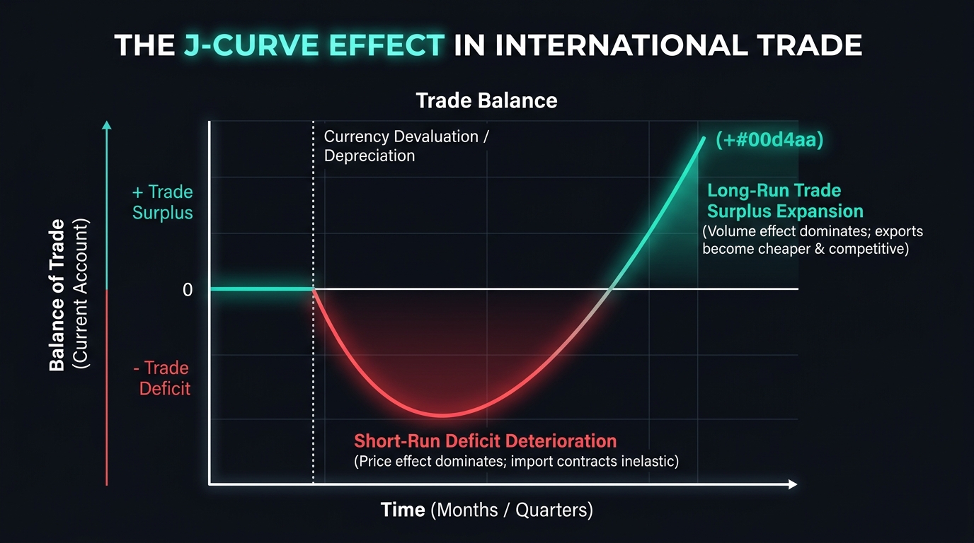
The J-Curve is an economic theory illustrating that a country's trade balance initially deteriorates following a currency depreciation or devaluation before rebounding and strengthening over time, tracing the shape of the letter 'J'.
What Is the J-Curve Effect?
The J-Curve is a prominent macroeconomic concept that describes the temporal response of a country’s balance of trade (the current account) following a sudden depreciation or deliberate devaluation of its national currency.
According to economic theory, a weaker currency makes a country’s exports cheaper for foreign buyers while making foreign imports more expensive for domestic consumers, which should naturally correct a national trade deficit. However, in real-world economics, the trade balance does not improve immediately. Instead, it initially worsens, plunging into an even deeper deficit before eventually recovering and climbing into a healthy surplus. When plotted on a time-series graph, this trajectory traces the visual contour of the capital letter “J”.
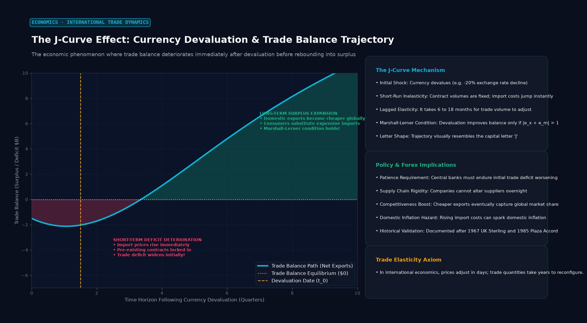 Figure: The economic phenomenon where trade balance deteriorates immediately after devaluation before rebounding into surplus
The Two Chronological Phases of the J-Curve
The counter-intuitive shape of the J-Curve is driven by a mismatch between short-run price adjustments and long-run volume adjustments:
Phase 1: Short-Run Deterioration (Price Effect Dominates)
Immediately following a currency depreciation, trade volumes remain rigid due to pre-existing commercial contracts and consumer habits:
- Locked-In Contracts: Importers and exporters operate on 3-month to 12-month pre-negotiated purchase agreements. Domestic businesses must honor shipments of foreign raw materials, energy, and components ordered before the devaluation.
- Inelastic Demand: Because domestic consumers cannot instantly switch from foreign fuel, electronics, or industrial machinery to domestic substitutes, the quantity of imports demanded remains virtually unchanged.
- Inflated Import Costs: Because the domestic currency has weakened, paying for that same fixed physical volume of foreign imports requires significantly more domestic currency. Consequently, the national import bill expands immediately, while export revenues have not yet grown, causing the trade deficit to widen sharply.
Phase 2: Long-Run Improvement (Volume Effect Dominates)
Over an extended adjustment horizon—typically spanning 6 to 18 months—market participants adjust their behavior as price elasticity takes effect:
- Import Substitution: Domestic manufacturers and consumers replace expensive imported goods with locally produced alternatives, causing the physical volume of imports to decline.
- Surging Export Competitiveness: Foreign consumers and multinational supply chains recognize that the country’s exports are now substantially cheaper in foreign currency terms. Global purchase orders surge.
- Surplus Realization: The expanding volume of exports combined with contracting import volumes overpowers the initial price shock, steering the trade balance into a durable surplus.
The Mathematical Foundation: The Marshall-Lerner Condition
The economic mechanism governing the J-Curve is formalized by the Marshall-Lerner Condition, formulated by economists Alfred Marshall and Abba Lerner.
The condition states that for a currency depreciation to successfully improve a nation’s trade balance in the long run, the sum of the price elasticity of demand for exports ($\varepsilon_x$) and the price elasticity of demand for imports ($\varepsilon_m$) must be greater than 1:
$$|\varepsilon_x + \varepsilon_m| > 1$$
Where:
- $\varepsilon_x$ = Percentage change in export quantity demanded divided by percentage change in price
- $\varepsilon_m$ = Percentage change in import quantity demanded divided by percentage change in price
Timeline of Elasticity:
- Short Run (0 to 6 Months):   |ε_x + ε_m| < 1  ===> Inelastic; Trade Deficit Deepens
- Long Run  (6 to 18 Months):  |ε_x + ε_m| > 1  ===> Elastic; Trade Balance Recovers
In the short run, trade elasticity is below 1 because neither buyers nor sellers can alter physical production pipelines quickly. Only when long-run elasticity surpasses 1 does the Marshall-Lerner condition hold true, driving the upward arm of the J-Curve.
Real-World Case Studies
1. The Plaza Accord and the US Dollar (1985–1987)
Following the landmark Plaza Accord in September 1985, the G5 nations agreed to depreciate the overvalued US Dollar to alleviate the massive US trade deficit. Over the subsequent 18 months, the dollar plunged by more than 40% against the Japanese Yen and German Deutsche Mark. Yet, throughout 1986, the US current account deficit expanded to historic highs, sparking public panics that the policy had failed. By late 1987 and 1988, the volume effect finally took hold: US manufacturing exports surged, and the trade deficit narrowed dramatically, validating the J-Curve.
2. The Brexit Referendum and the British Pound (2016)
Following the June 2016 Brexit referendum, the British Pound (GBP) plummeted by 15% against the US Dollar and Euro. In the immediate aftermath, the UK trade deficit widened to multi-year records as the cost of imported food, fuel, and manufactured goods surged. It took nearly two years for British export volumes to capitalize on the competitive exchange rate and rebalance external accounts.
Trading Implications for Forex Participants
- Avoid Premature Trade Balance Bets: When a central bank devalues its currency to boost exports, macro traders must recognize that the immediate trade balance reports over the next 1 to 2 quarters will look alarming. Shorting the currency further based on widening short-term trade deficits often results in getting caught on the wrong side when the J-Curve inflects upward.
- Lagged Inflation Impulses: The initial downward stroke of the J-Curve imports immediate inflation. Central banks are often forced to maintain higher interest rates during this window to prevent imported inflation from embedding into domestic wage expectations.
Key Takeaways
- The J-Curve illustrates that a currency depreciation initially worsens a nation’s trade balance before improving it.
- In the short run, pre-existing trade contracts and price-inelastic demand inflate the national import bill.
- In the long run, consumers substitute imports and foreign demand for cheaper exports expands.
- The Marshall-Lerner condition ($|\varepsilon_x + \varepsilon_m| > 1$) mathematically dictates whether depreciation will ultimately create a trade surplus.
- Historical examples (1985 Plaza Accord, 2016 Brexit) confirm that the J-Curve adjustment typically requires 12 to 18 months to complete.
Frequently Asked Questions
Why does a currency depreciation make imports more expensive?
When a domestic currency depreciates, it takes more units of that currency to purchase one unit of foreign currency. Because foreign exporters invoice goods in foreign currency, domestic businesses and consumers must pay higher domestic prices for the exact same imported items.
Can a J-Curve fail to materialize?
Yes. If an economy lacks domestic industrial capacity to manufacture import substitutes (e.g., small island nations that must import 100% of their fuel and food), demand for imports remains permanently inelastic. In such cases, currency depreciation permanently worsens the trade deficit and stokes inflation without generating export expansion.
How long does the J-Curve cycle typically take to inflect upward?
Empirical macroeconomic studies suggest that the bottom of the J-Curve is typically reached between 6 and 9 months following the initial devaluation, with full trade balance recovery and surplus expansion unfolding over 12 to 24 months.
Ready to trade forex?
Open a free demo account with a regulated broker. Practice with virtual funds before risking real money.