Macroeconomics

Macroeconomics is the study of aggregate economic systems at regional, national, and global levels. Rather than examining individual consumer choices or single corporate pricing strategies (the domain of microeconomics), macroeconomics analyzes systemic economic indicators: gross domestic product (GDP), economy-wide inflation rates, national unemployment levels, sovereign fiscal balances, and foreign exchange movements.

For institutional market participants, central bankers, and foreign exchange traders, macroeconomics provides the analytical foundation for understanding market regimes. Capital allocation across global asset classes (currencies, sovereign debt, corporate equities, and physical commodities) is determined by macro drivers such as central bank interest rate cycles, government debt expansion, terms of trade, and productivity growth.

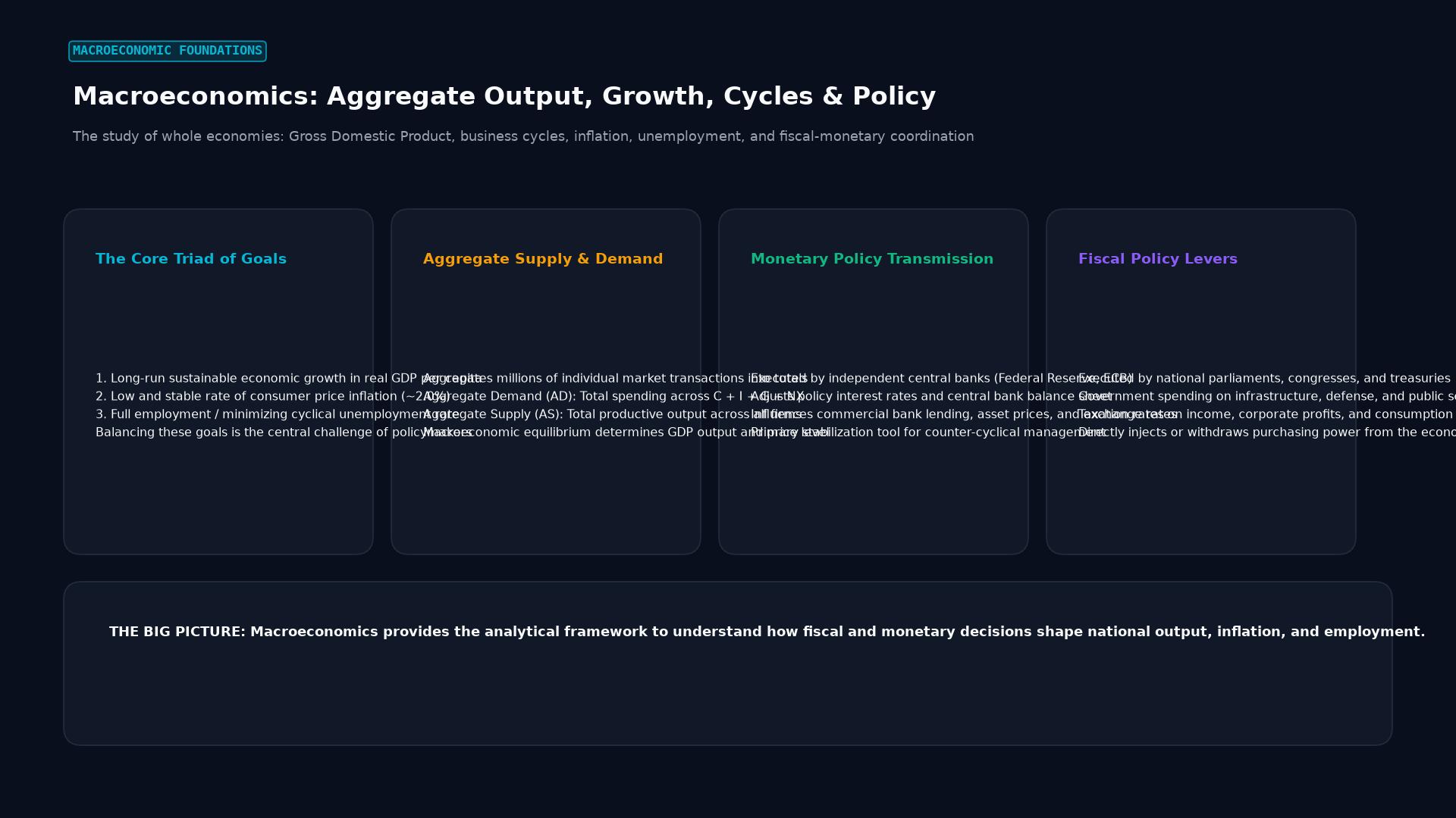Figure: The study of whole economies: Gross Domestic Product, business cycles, inflation, unemployment, and fiscal-monetary coordination

Historical and Theoretical Evolution

The modern discipline of macroeconomics was forged in response to systemic market crises. Its theoretical framework has evolved through distinct intellectual paradigms:

1. Classical Economics and Say’s Law

Prior to the 1930s, classical economists such as Adam Smith, David Ricardo, and Jean-Baptiste Say viewed the aggregate economy as a self-correcting system. Say’s Law posited that “supply creates its own demand,” implying that general gluts of unsold goods and prolonged involuntary unemployment were theoretically impossible. Flexible prices and wages were assumed to restore full employment equilibrium automatically.

2. The Keynesian Revolution

The Great Depression of the 1930s exposed the limitations of classical assumptions as unemployment persisted above 20% in the United States and Europe for years. In 1936, British economist John Maynard Keynes published The General Theory of Employment, Interest and Money, introducing modern macroeconomics. Keynes argued that:

• Aggregate demand ($AD$) determines the level of economic activity and employment.
• Nominal wages and prices are “sticky” downward due to contracts, institutional norms, and labor unions.
• In a liquidity trap, private investment collapses as market participants hoard cash.
• Countercyclical fiscal policy (deficit-financed government spending) is necessary to close the output gap and restore full employment.

3. Monetarism and the Chicago School

During the 1970s, Keynesian consensus faltered under the emergence of “stagflation” (simultaneous high inflation and stagnant growth). Led by Milton Friedman, monetarists challenged the efficacy of fiscal fine-tuning, asserting that “inflation is always and everywhere a monetary phenomenon.” Friedman demonstrated that the money supply ($M$) dictates nominal GDP over the long run, and that central banks should follow transparent money growth rules rather than discretionary interventions.

4. The New Classical Counter-Revolution and Lucas Critique

In the late 1970s, Robert Lucas, Thomas Sargent, and Edward Prescott introduced Rational Expectations. The Lucas Critique proved that historical statistical correlations between macro variables (such as the traditional Phillips Curve trade-off between inflation and unemployment) collapse when policy rules change, because economic agents adapt their forward-looking behavior. Real Business Cycle (RBC) theory argued that economic fluctuations are driven primarily by real technology and productivity shocks rather than monetary disturbances.

5. The New Keynesian Synthesis

The contemporary operating consensus in central banking combines New Classical microeconomic foundations (rational expectations and intertemporal optimization) with Keynesian nominal rigidities (monopolistic competition and Calvo sticky pricing). This framework forms the mathematical basis for Dynamic Stochastic General Equilibrium (DSGE) models used by the Federal Reserve, the European Central Bank, and the Bank of England.

                    EVOLUTION OF MACRO PARADIGMS
                    
Period      Dominant School      Key Assumption            Primary Tool
----------------------------------------------------------------------------------
Pre-1930s   Classical Economics  Flexible wages & prices   Free-market adjustment
1930s-1960s Keynesian Economics  Sticky wages, demand gap  Fiscal deficit stimulus
1970s-1980s Monetarism           Money supply drives price Money supply targets
1980s-1990s New Classical / RBC  Rational expectations     Supply-side reforms
2000s-Pres. New Keynesian        Sticky prices + DSGE      Inflation targeting / Rates

Core Quantitative Frameworks and Equations

Macroeconomics employs explicit accounting identities and behavioural equations to model national economic activity:

1. The National Income Identity (Expenditure Approach)

Gross Domestic Product ($Y$) represents the total market value of all final goods and services produced within a nation during a specified period:

$$Y = C + I + G + (X - M)$$

Where:

• $C$ is private household consumption expenditure.
• $I$ is gross private domestic capital investment (machinery, real estate, inventories).
• $G$ is government consumption and gross infrastructure investment.
• $X$ is gross exports of goods and services.
• $M$ is gross imports of goods and services, making $(X - M)$ net exports ($NX$).

From the national savings-investment identity, domestic investment must equal national savings plus foreign capital inflows:

$$S + (T - G) = I + NX$$

$$(S - I) + (T - G) = NX$$

This identity illustrates the “twin deficits” phenomenon: when a government runs a fiscal deficit ($G > T$) and domestic private savings ($S$) fail to cover private investment ($I$), the nation must run a current account trade deficit ($NX < 0$), importing foreign capital to balance the national accounts.

2. The Quantity Theory of Money

Milton Friedman revived the classical Fisher Equation of Exchange to explain nominal price determination:

$$M \times V = P \times Y$$

Where:

• $M$ is the aggregate nominal money supply (e.g., M2).
• $V$ is the velocity of money (the frequency with which a unit of currency changes hands).
• $P$ is the aggregate price level (GDP deflator).
• $Y$ is real gross domestic output.

Assuming velocity ($V$) and real potential output ($Y$) are determined by structural, institutional factors in the long run, sustained growth in the money supply ($\Delta M$) directly drives changes in the price level ($\Delta P$), producing inflation:

$$% \Delta M + % \Delta V \approx % \Delta P + % \Delta Y$$

3. The Taylor Rule for Central Bank Rates

Formulated by John B. Taylor in 1993, the Taylor Rule describes how central banks adjust their short-term nominal policy rate ($i_t$) in response to deviations of inflation and output from their targets:

$$i_t = r^* + \pi_t + \alpha_\pi (\pi_t - \pi^) + \alpha_y (y_t - y^)$$

Where:

• $r^*$ is the equilibrium real natural rate of interest ($r$-star).
• $\pi_t$ is the current rate of inflation.
• $\pi^*$ is the central bank inflation target (typically 2.0%).
• $y_t - y^*$ is the output gap (the percentage difference between actual real GDP and potential GDP).
• $\alpha_\pi$ and $\alpha_y$ are policy responsiveness coefficients (standard values: $\alpha_\pi = 0.5$, $\alpha_y = 0.5$).

The Taylor Principle stipulates that $\alpha_\pi > 0$ (implying the total coefficient on inflation is $1 + \alpha_\pi > 1.0$). When inflation rises by 100 basis points, the central bank must raise nominal rates by more than 100 basis points to increase the real interest rate ($r = i - \pi$), cooling aggregate demand.

4. The Expectations-Augmented Phillips Curve

Developed by Edmund Phelps and Milton Friedman, this equation models the relationship between inflation and unemployment:

$$\pi_t = \pi_t^e - \beta (u_t - u_n) + \nu_t$$

Where:

• $\pi_t$ is realized inflation.
• $\pi_t^e$ is expected inflation.
• $u_t$ is the actual unemployment rate.
• $u_n$ is the Natural Rate of Unemployment (or Non-Accelerating Inflation Rate of Unemployment, NAIRU).
• $\beta$ is the sensitivity parameter.
• $\nu_t$ represents supply shocks (such as global energy or food price surges).

When the labor market operates beyond capacity ($u_t < u_n$), wage pressures push inflation above expectations.

       EXPECTATIONS-AUGMENTED PHILLIPS CURVE
       
Inflation
  (pi)
   ^
   |        Long-Run Phillips Curve (LRPC)
   |                    |
   |                    |  Short-Run Phillips Curve (High Inflation Exp.)
   |             \      |      /
   |              \     |     /
   |               \    |    /
   |                \   |   /  Short-Run Phillips Curve (Low Inflation Exp.)
   |                 \  |  /
   |                  \ | /
   +--------------------+------------------------>
   0                   u_n (NAIRU)             Unemployment (u)

Macroeconomics in Foreign Exchange and Global Trading

For currency traders, macroeconomic indicators dictate directional exchange rate trends through three fundamental channels:

1. Interest Rate Parity and Yield Differentials

Capital flows toward currencies offering higher real risk-adjusted yields. Traders monitor the short-term yield differential between sovereign bonds:

$$\text{Yield Spread} = (i_{\text{domestic}} - \pi_{\text{domestic}}) - (i_{\text{foreign}} - \pi_{\text{foreign}})$$

When a central bank tightens monetary policy faster than its peers, the domestic currency tends to appreciate as institutional investors execute carry trades, borrowing in low-yielding funding currencies (e.g., JPY, CHF) to purchase higher-yielding sovereign assets (e.g., USD, AUD).

2. Terms of Trade and Current Account Dynamics

Export-driven economies that experience positive terms-of-trade shocks (such as Australia or Canada during commodity supercycles) benefit from increased foreign demand for their currencies to settle trade contracts. Conversely, persistent trade deficits require continuous capital account surpluses (foreign investment inflows) to prevent currency depreciation.

3. Economic Indicator Calendar

Macro traders track economic data releases against consensus expectations:

• Leading Indicators: Purchasing Managers’ Index (PMI), yield curve slope, consumer confidence indices, building permits.
• Coincident Indicators: Non-Farm Payrolls (NFP), industrial production, retail sales.
• Lagging Indicators: Headline Consumer Price Index (CPI), corporate earnings reports, national unemployment rate.

Real-World Case Study: The 2021-2023 Global Inflation Shock

The macroeconomic cycle following the 2020 pandemic provides a modern demonstration of fiscal stimulus, monetary expansion, supply constraints, and subsequent policy tightening.

+--------------------------------------------------------------------+
|           THE 2020-2023 GLOBAL MACROECONOMIC SEQUENCE              |
+--------------------------------------------------------------------+
| 1. Exogenous Shock (2020): Global shutdowns; real GDP contracts    |
|    at double-digit annualized rates.                               |
| 2. Fiscal and Monetary Stimulus: Over $5 trillion in US fiscal     |
|    packages (CARES, ARPA); Fed expands balance sheet by $4.5T.     |
| 3. Money Supply Acceleration: US M2 growth exceeds 27% YoY (record)|
| 4. Supply Shocks (2021-2022): Semiconductor shortages, shipping   |
|    container bottlenecks, Ukrainian war energy shock.              |
| 5. Inflation Surge (2022): US CPI reaches 9.1%, Eurozone reaches   |
|    10.6% (highest in 40 years).                                    |
| 6. Aggressive Central Bank Tightening: Federal Reserve hikes rates |
|    525 bps; ECB exits negative rates, lifting deposit rate to 4.0%.|
| 7. FX Repercussions: USD Index (DXY) hits 20-year high at 114.7;   |
|    EUR drops below USD parity; JPY weakens past 150.               |
+--------------------------------------------------------------------+

Between 2020 and 2021, major governments deployed massive countercyclical fiscal deficits while central banks purchased sovereign debt through quantitative easing. This coordinated expansion stimulated aggregate demand ($AD$) at the precise moment aggregate supply ($AS$) was impaired by broken supply chains and factory shutdowns.

As predicted by the Quantity Theory of Money and the AD-AS framework, this imbalance caused consumer prices to accelerate rapidly. In 2022, headline inflation reached 9.1% in the United States and 10.6% in the Eurozone. Central banks responded with the fastest rate-hiking cycle in four decades. The Federal Reserve raised the Federal Funds Rate from 0.00-0.25% to 5.25-5.50% in eighteen months.

In foreign exchange markets, the aggressive pace of Fed tightening widened the US-Japan interest rate differential, causing the Japanese yen (where the Bank of Japan maintained yield curve control at 0.00%) to depreciate from 115 to over 151 JPY per USD. Meanwhile, the euro plunged below parity against the US dollar in September 2022 as Europe suffered a terms-of-trade collapse caused by surging imported natural gas prices.

Frequently Asked Questions

What is the core difference between microeconomics and macroeconomics?

Microeconomics focuses on individual decision-makers within an economy: individual consumers maximizing utility, businesses setting production volumes and prices, and the equilibrium of single product markets. Macroeconomics examines the aggregate economy as a complete system: total national output (GDP), aggregate price inflation, overall unemployment rates, national balance of payments, and government fiscal and monetary policies.

How does central bank quantitative easing (QE) affect the macro economy?

Quantitative easing is an unconventional monetary policy tool used when benchmark interest rates reach the zero lower bound. The central bank creates electronic bank reserves to purchase long-duration government bonds and mortgage-backed securities directly from commercial banks. This action reduces long-term benchmark yields, compresses credit spreads, inflates asset valuations, and increases commercial bank liquidity reserves, encouraging lending and capital investment.

Why do currency traders monitor the Purchasing Managers’ Index (PMI) so closely?

The Purchasing Managers’ Index (PMI) is considered a primary leading economic indicator. Based on monthly surveys of senior purchasing executives across manufacturing and services sectors, the PMI measures forward-looking business conditions: new customer orders, factory output, employment changes, supplier delivery times, and inventory levels. Because a reading above 50 signals economic expansion and a reading below 50 signals contraction, PMI releases often foreshadow future shifts in GDP growth and central bank rate policy before official government GDP data is published.