Quantitative Analysis — Forex Dictionary Definition

What Is Quantitative Analysis?

In modern institutional finance, quantitative analysis (quant analysis) is the application of mathematical, statistical, and econometric methodologies to financial market data. Rather than relying on subjective human intuition, qualitative company narratives, or visual chart reading, quantitative analysts (commonly called quants) build algorithmic models, statistical arbitrage engines, and systematic execution algorithms to identify repeatable market anomalies and extract risk-adjusted returns (alpha).

Pioneered by mathematicians and physicists—most notably Jim Simons of Renaissance Technologies, Fischer Black, Myron Scholes, and Edward Thorp—quantitative analysis now drives over 70% of total daily trading volume across global equity and foreign exchange markets.

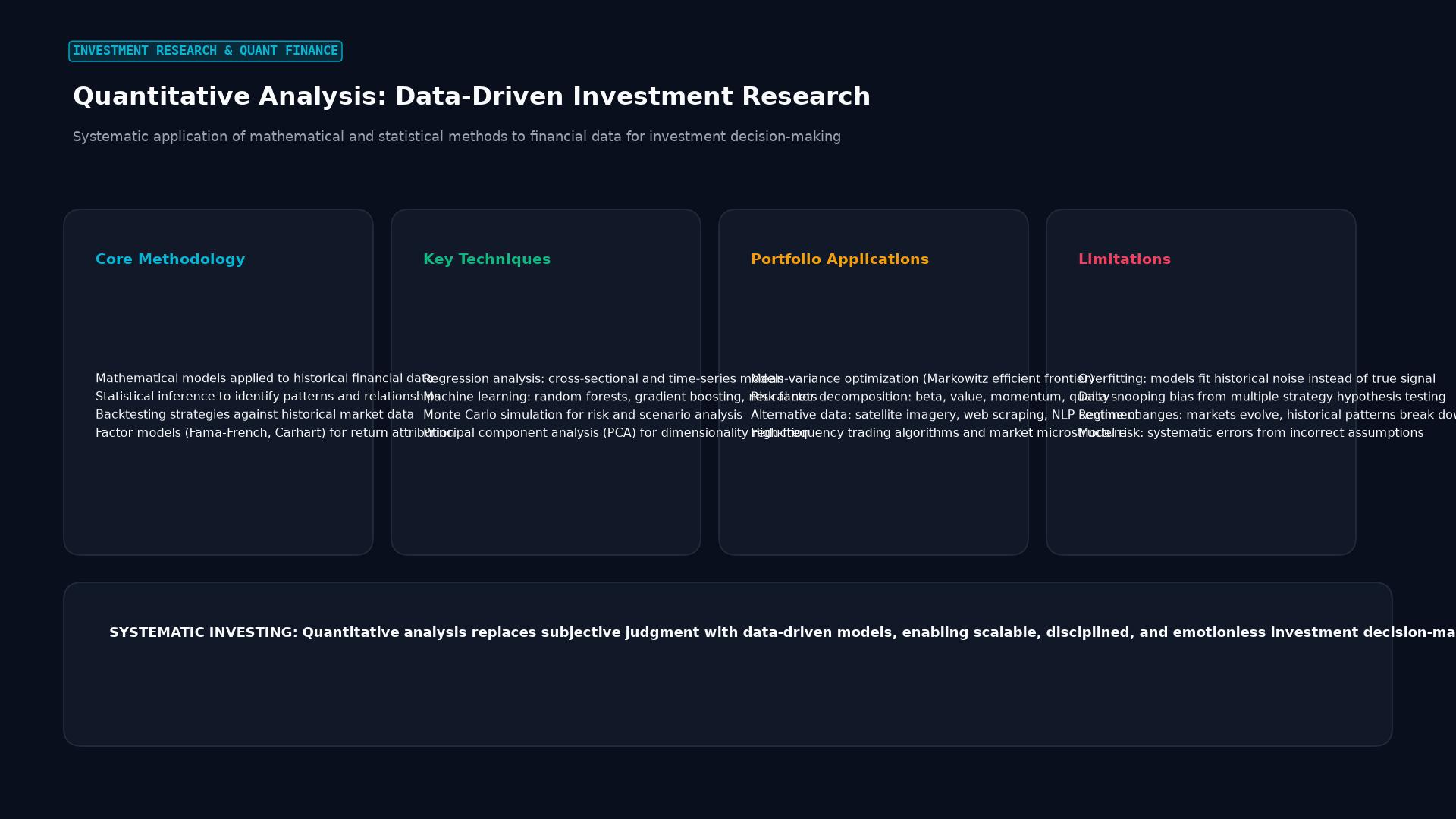Quantitative Analysis: Data-Driven Investment Research Figure: Systematic application of mathematical and statistical methods to financial data for investment decision-making

Core Methodologies in Quantitative Finance

Institutional quant funds deploy sophisticated mathematical frameworks across distinct trading domains:

1. Statistical Arbitrage (StatArb) and Pairs Trading

Quants utilize advanced time-series econometrics (such as the Engle-Granger Cointegration Test) to identify two historically correlated assets whose price spread has temporarily widened:

When the spread between two cointegrated currency pairs (or equities) exceeds a 2-standard-deviation threshold ($Z$-score $> 2.0$), the algorithm automatically shorts the outperforming asset and buys the underperforming asset, profiting when the spread reverts to the historical mean: $$Z = \frac{\text{Spread}t - \mu{\text{Spread}}}{\sigma_{\text{Spread}}}$$

2. Multi-Factor Modeling

Originating from the Capital Asset Pricing Model (CAPM) and expanded by the Fama-French 5-Factor Model, quantitative equity desks decompose portfolio returns into systematic factor exposures:

Value Factor: Cheap assets outperforming expensive assets.
Momentum Factor: Assets with strong 12-month returns continuing to outperform.
Low Volatility Factor: Statistically lower beta assets generating superior risk-adjusted returns.
Quality & Size Factors: High return on equity (ROE) and small-cap premia.

3. High-Frequency Trading (HFT) and Microstructure

HFT quants model the millisecond and microsecond dynamics of the limit order book (CLOB). By analyzing order flow toxicity, bid-ask imbalances, and market depth queues, algorithms capture fractions of a cent per share across millions of daily transactions while maintaining market-neutral books.

4. Risk Modeling: Monte Carlo and Value at Risk (VaR)

Quantitative risk managers run hundreds of thousands of simulated market paths (Monte Carlo simulations) incorporating non-normal fat-tailed distributions (such as Student’s t or Pareto distributions) to stress-test institutional balance sheets against severe market shocks.

Comparison of Analytical Approaches

The structural differences between traditional and quantitative methodologies include:

Feature	Fundamental Analysis	Traditional Technical Analysis	Quantitative Analysis
Data Source	Financial statements, earnings, GDP, CPI prints.	Price, volume, visual candlesticks, chart patterns.	Order book ticks, time series, alternative data (satellite, web traffic).
Decision Engine	Human portfolio manager discretion.	Discretionary trader pattern recognition.	Automated code execution (Python, C++, Rust).
Emotional Bias	Vulnerable to cognitive bias and narrative trap.	High emotional friction (fear, greed, revenge trading).	Zero: Algorithms execute strictly according to mathematical rules.
Scalability	Low; a human analyst can monitor 20–30 stocks.	Medium; scanner-assisted discretionary monitoring.	Virtually Infinite: Models scan tens of thousands of instruments in milliseconds.
Primary Failure Mode	Value trap (cheap stock stays cheap indefinitely).	High false-positive rate; subjective pattern interpretation.	Overfitting (Curve-Fitting) and regime change failure.

The Greatest Danger: Backtest Overfitting and Regime Shift

While quantitative analysis eliminates human emotional error, it introduces dangerous quantitative vulnerabilities:

1. Backtest Overfitting (Data Snooping)

If a researcher tests thousands of mathematical indicator combinations against historical data, they will inevitably discover a parameter set that produces an extraordinary backtested Sharpe Ratio purely by random chance. When deployed into live forward markets, overfitted models almost invariably collapse.

2. Regime Shift Failures

Quantitative models are calibrated on historical training data. When unprecedented macroeconomic shocks occur (such as the 2007 subprime mortgage freeze, the 2020 pandemic lockdowns, or historic central bank emergency interventions), historical correlations break down, causing statistical arbitrage algorithms to suffer catastrophic drawdowns.

       THE QUANTITATIVE BREAKDOWN IN REGIME SHIFTS
       
  Historical Normal Regime ---> Model Calibrated: Assets A & B Correlated (+0.92)
                                                 |
  Black Swan Event Occurs  ---> Macro Shock: Correlation Inverts (-0.85)
                                                 |
  Algorithm Keeps Buying Dip <--- Assuming Spread Must Mean-Revert!
                                                 |
  Catastrophic Margin Liquidation ---> Severe Capital Loss

Real-World Case Study: The Quant Meltdown of August 2007

In the second week of August 2007, prior to the broader subprime crisis, global financial markets experienced the legendary “Quant Meltdown”:

The Setup: Hundreds of quantitative hedge funds (including Goldman Sachs’ Global Alpha Fund, Highbridge, and Renaissance) were running similar long-short statistical equity factor models.
The Unwind: A multi-strategy investment fund facing liquidity pressures in subprime mortgage derivatives began liquidating portions of its equity portfolio to raise cash.
The Cascade: The fire-sale caused the “value” factors owned by quants to plummet, while the “short” factors they had sold short rallied. As quantitative risk management models triggered automated stop-losses, dozens of algorithms simultaneously executed the exact same liquidation trades.
The Result: Top-performing quantitative hedge funds suffered unprecedented 20% to 30% drawdowns within three days, losing billions in a market-neutral environment. The event demonstrated that when quants utilize similar data and risk parameters, crowded factor positioning can transform uncorrelated strategies into systemic liquidity contagion.

Frequently Asked Questions

What programming languages are essential for quantitative analysis?

Python is the industry standard for quantitative research, data cleaning, backtesting, and machine learning (using libraries like NumPy, Pandas, Scikit-Learn, and PyTorch). C++ and Rust are universally required for low-latency high-frequency trading (HFT) and live production execution engines where microsecond execution speed is paramount.

Can retail traders use quantitative analysis?

Yes. Retail traders increasingly deploy quantitative techniques by backtesting algorithmic trading strategies using platforms like MetaTrader (MQL5), TradingView (Pine Script), or custom Python frameworks. Focusing on objective mathematical entry rules, automated position sizing, and statistical edge calculation elevates retail performance above subjective discretionary trading.

What is the difference between a Quant Researcher and a Quant Developer?

Quant Researcher: Focuses on mathematics, statistics, and financial economics—discovering new mathematical anomalies, analyzing market signals, and engineering trading strategies.
Quant Developer: Focuses on computer science and software architecture—building ultra-low-latency execution engines, managing data feeds, and optimizing algorithmic speed.