Trading Model

What Is a Trading Model?

A trading model is a formalized, systematic framework that translates mathematical, statistical, or economic theories into automated or semi-automated trading rules. Unlike discretionary trading—which depends on subjective trader intuition and cognitive heuristics—a trading model operates on explicit, deterministic logic: given a specific input vector of market data $X_t$, the model deterministically produces an output state $S_t$ dictating entry, exit, position sizing, or portfolio rebalancing.

In institutional asset management, hedge funds, and proprietary trading desks, trading models underpin systematic macro strategies, statistical arbitrage, trend following (CTAs), and high-frequency market making. These models eliminate behavioral biases, enforce rigorous risk budgets, and allow strategies to be scientifically backtested, validated, and optimized across decades of historical tick or bar data.

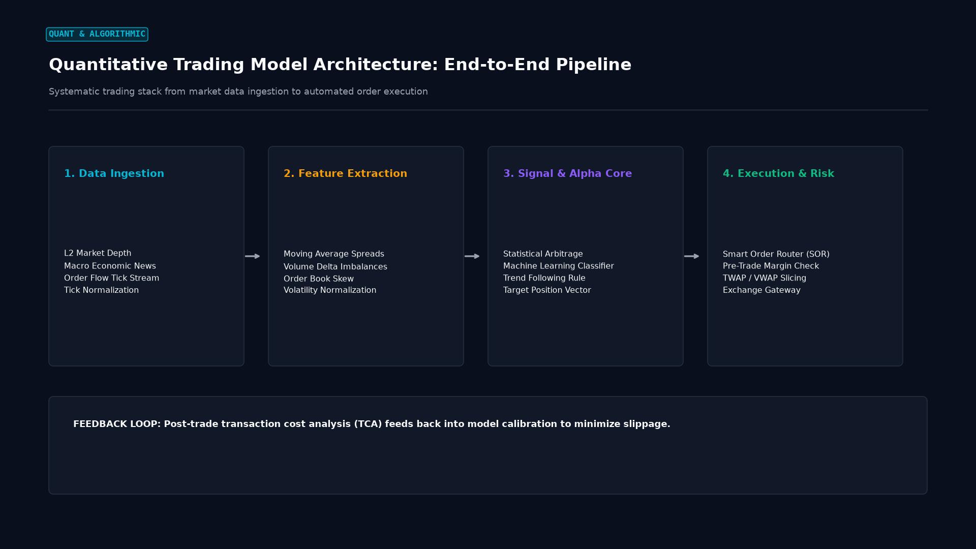Figure: Algorithmic trading engine pipeline: market data ingestion, feature extraction, alpha signal generation, pre-trade risk filters, and smart order routing.

---

Mathematical Foundations & Performance Metrics

A robust trading model requires quantitative benchmarks to evaluate predictive alpha, risk-adjusted returns, and resilience against parameter overfitting.

1. The Signal Function

At its core, a systematic model maps time-series features $X_t$ with parameter set $\theta$ to an active target position $w_t \in [-1, 1]$:

$$w_t = g\left( \sum_{i=1}^{k} \beta_i f_i(X_t) \right)$$

Where $w_t = +1$ represents maximum long exposure, $w_t = -1$ represents maximum short exposure, and $w_t = 0$ represents a neutral cash state.

2. Risk-Adjusted Return Metrics

The Sharpe Ratio

The annualized Sharpe Ratio quantifies excess return earned per unit of total portfolio volatility:

$$\text{Sharpe Ratio} = \frac{\mathbb{E}[R_p - R_f]}{\sigma_p} \times \sqrt{N}$$

Where $R_p$ is portfolio return, $R_f$ is the risk-free rate, $\sigma_p$ is standard deviation, and $N$ is the annualization factor ($N = 252$ for daily equities/FX, $N = 365$ for 24/7 crypto).

The Information Ratio (IR)

Used by institutional multi-asset managers to evaluate alpha generation relative to a benchmark index $R_b$:

$$\text{Information Ratio} = \frac{\mathbb{E}[R_p - R_b]}{\sigma(R_p - R_b)} = \frac{\alpha}{\omega}$$

Where $\omega = \sigma(R_p - R_b)$ denotes tracking error.

3. Walk-Forward Optimization (WFO) Efficiency

To prevent curve-fitting (optimizing parameters to historical noise rather than genuine market structure), institutional modelers employ out-of-sample walk-forward analysis:

$$\text{WFO Efficiency Ratio} = \left( \frac{\text{Sharpe}{\text{out-of-sample}}}{\text{Sharpe}{\text{in-sample}}} \right) \times 100$$

A ratio above $60%$ indicates robust parameter stability, whereas a ratio below $30%$ signals severe overfitting and likely real-world strategy failure.

---

Major Trading Model Archetypes

Systematic trading models are categorized by investment horizon, mathematical formulation, and underlying economic thesis:

Model Classification	Core Premise	Primary Alpha Drivers	Average Holding Horizon
Trend Following (CTA)	Capitalizes on persistent multi-month price trends driven by behavioral underreaction and macroeconomic regimes.	Moving average envelopes, breakout channels (Donchian), ATR filters.	Weeks to several months.
Mean Reversion / Stat-Arb	Exploits temporary asset price deviations from their historical equilibrium or cointegrated relationships.	Johansen cointegration, Ornstein-Uhlenbeck processes, Bollinger bands.	Minutes to a few days.
High-Frequency Market Making	Captures the bid-ask spread while maintaining a delta-neutral inventory.	Avellaneda-Stoikov inventory models, order flow toxicity (VPIN).	Sub-second to minutes.
Machine Learning / Multi-Factor	Detects non-linear interactions across hundreds of fundamental, technical, and macroeconomic features.	Gradient Boosted Decision Trees (XGBoost), Recurrent Neural Networks, Ridge regression.	Hours to weeks.

---

Overfitting vs. Robustness in Model Design

The single greatest point of failure in trading model development is data mining bias. When a modeler tests thousands of indicator permutations, standard statistical significance thresholds ($p < 0.05$) fail due to the multiple testing problem.

Overfitted Model (Curve-Fitted to Noise)
In-Sample Equity Curve:  /------------------ (Sharpe 4.2 - Unrealistically smooth)
Out-of-Sample Reality:   \________/\_______/ (Instant collapse in live trading)

Robust Institutional Model (Economic Logic + Out-of-Sample Validation)
In-Sample Performance:   /---\_/\--/\_/-/\-- (Sharpe 1.6 - Realistic drawdowns)
Out-of-Sample Reality:   /--\_/\--/\_/-/\--- (Consistent, durable alpha)

Institutional Defense Mechanisms:

1. White’s Reality Check & Hansen’s Superior Predictive Ability: Adjusts standard error thresholds for the number of backtested strategy variations.
2. Deflated Sharpe Ratio (Bailey & López de Prado): Discounts nominal Sharpe ratios based on sample length, skewness, kurtosis, and the total number of trial iterations.
3. Execution Slippage & Latency Penalties: Incorporates realistic transaction cost models ($TC = \text{Half-Spread} + \text{Commission} + \text{Market Impact}$) directly into backtesting engines.

---

Real-World Institutional Case Study: The August 2007 “Quant Quake”

In the second week of August 2007, several of the world’s most prestigious quantitative equity and multi-asset market-neutral hedge funds—including Goldman Sachs’ Global Alpha Fund, Renaissance Technologies, and Highbridge Capital—experienced unprecedented multi-sigma drawdowns within a 72-hour window.

The crisis occurred without any obvious macroeconomic catalyst or broad stock market crash. Instead, the driver was structural model correlation. Over the preceding decade, hundreds of quantitative funds had independently developed multi-factor statistical arbitrage models optimizing for similar predictive signals: value (book-to-price), momentum, and earnings quality.

[August 6-9, 2007: The Crowded Factor Deleveraging Cascade]
Subprime Mortgage Losses at Multi-Strategy Fund
                  |
                  v
Forced Liquidation of Liquid Equity Portfolio to Meet Cash Demands
                  |
                  v
Fire-Sale of Quant-Favored Long Positions / Buyback of Quant Shorts
                  |
                  v
Factor Returns Breakdown: Value and Momentum Factors Collapse 30+ Standard Deviations
                  |
                  v
Automated Risk Engines Across All Quant Funds Breach VaR Limits Simultaneously
                  |
                  v
Synchronized Algorithmic Deleveraging: Cascading Liquidation across Wall Street

Because every fund’s risk model dictated immediate exposure reduction when Value at Risk (VaR) limits were breached, automated algorithms began dumping the same long assets and buying back the same short assets simultaneously. This historic event demonstrated that a trading model cannot be evaluated in a vacuum; models with identical mathematical logic create systemic liquidity feedback loops when aggregated across capital markets.

---

Frequently Asked Questions

What is the difference between an in-sample and out-of-sample test?

An in-sample dataset is the historical segment of price data used to discover patterns, calibrate parameters, and train the trading model. The out-of-sample dataset represents unobserved data strictly isolated from the training phase. Testing a model on out-of-sample data verifies whether the strategy possesses authentic generalizable predictive power or simply memorized historical market noise.

How does walk-forward analysis improve model validation?

Walk-forward analysis slices historical market data into multiple overlapping training (in-sample) and testing (out-of-sample) time windows. By re-optimizing parameters on window $N$ and immediately testing on window $N+1$, it simulates how the model would have dynamically adapted to evolving market regimes over time, providing a realistic estimate of live operational performance.

Can quantitative trading models eliminate market risk?

No. While quantitative models systematically minimize emotional biases and enforce rigid position-sizing rules, they remain susceptible to structural regime changes, tail-risk events, model specification errors, and systemic factor crowding. Effective risk management requires continuous human oversight and stress-testing under extreme macroeconomic dislocations.