CAGR - Compound Annual Growth Rate

What Is Compound Annual Growth Rate (CAGR)?

In investment finance and trading performance analysis, the Compound Annual Growth Rate (CAGR) represents the geometric annualized rate of return required for an investment to grow from its initial starting balance to its final ending balance over a specified timeframe greater than one year, under the assumption that all capital gains, dividends, and profits are compounded and reinvested at the conclusion of each period.

CAGR is not an actual raw accounting return that occurs consistently in any single isolated year. Instead, it is a representational mathematical smoothing metric. It illustrates the steady, constant annual percentage rate at which an asset would have expanded if it had grown at a frictionless, uniform pace without interim market turbulence or cyclical drawdowns.

Whether evaluating automated trading systems (Expert Advisors), institutional hedge fund track records, corporate revenue expansion, or long-term currency portfolio returns, CAGR serves as the universal global benchmark for performance comparison.

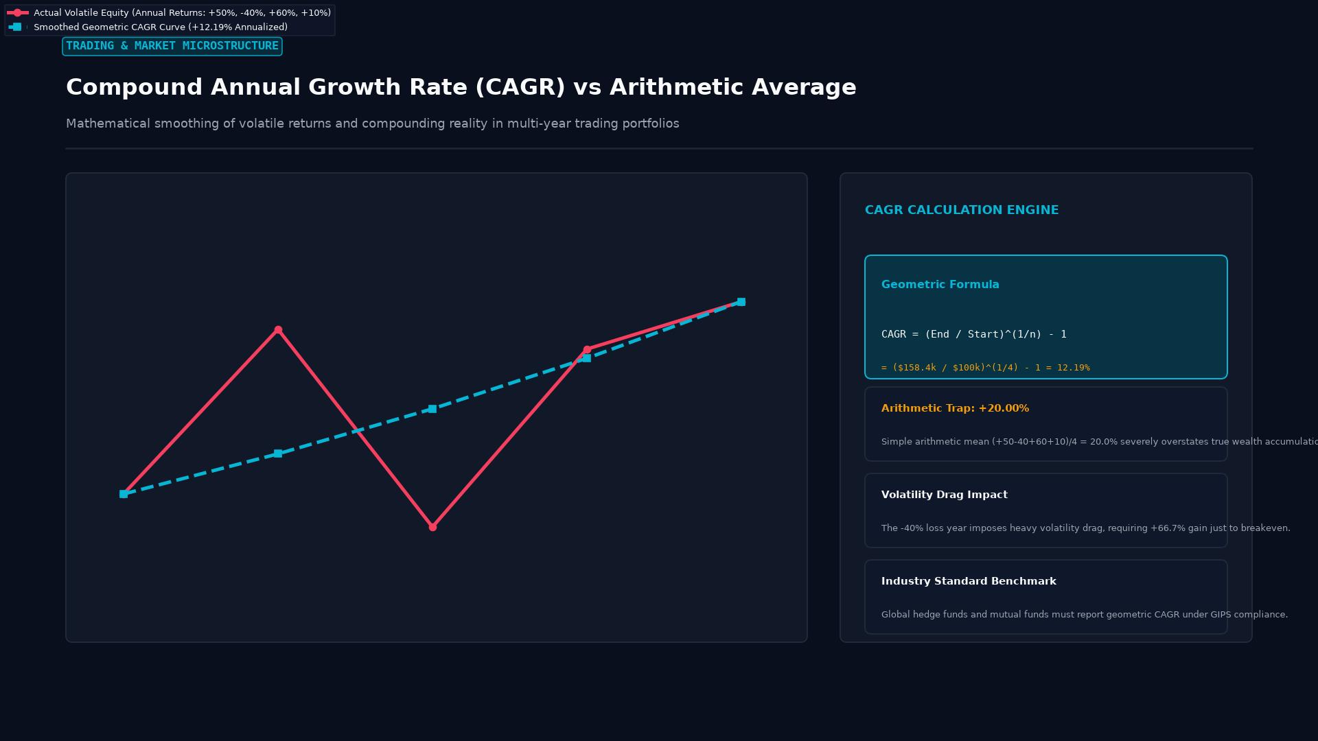Figure: Geometric CAGR smoothing of multi-year portfolio returns: illustrating the impact of volatility drag and the mathematical flaw of simple arithmetic averages.

The Mathematical Formula for CAGR

The mathematical calculation of CAGR requires only three data points: the initial principal, the terminal balance, and the total elapsed time:

$$ \text{CAGR} = \left( \frac{V_{\text{final}}}{V_{\text{initial}}} \right)^{\frac{1}{n}} - 1 $$

Where:

• $V_{\text{final}}$ = Ending Portfolio Value
• $V_{\text{initial}}$ = Beginning Portfolio Value
• $n$ = Number of elapsed investment years (which can be expressed as a decimal for fractional years, such as 2.5 years for 30 months)

To express the result as a standard percentage, multiply the resulting decimal by 100.

Why CAGR Beats the Arithmetic Average: The “Volatility Drag” Flaw

Many novice investors mistakenly compute their average annual return by taking the simple arithmetic average of individual yearly returns (adding up each year’s percentage gain or loss and dividing by the number of years). In finance, relying on arithmetic averages produces dangerously misleading results due to the mathematical reality of volatility drag.

Consider a trading portfolio with an initial capital deposit of $100,000 over a two-year period:

• Year 1: The trader achieves a spectacular +100% gain. The portfolio balance surges to $200,000.
• Year 2: The trader suffers a severe -50% loss. The portfolio collapses back to $100,000.

The Arithmetic Distortion:

$$ \text{Arithmetic Average Return} = \frac{(+100%) + (-50%)}{2} = \frac{+50%}{2} = +25.0% \text{ per year} $$

A fund manager marketing this track record could dishonestly claim an “average annual return of 25%.” In economic reality, the investor ended Year 2 with the exact same $100,000 they started with—achieving zero actual profit!

The True Geometric Reality (CAGR):

$$ \text{CAGR} = \left( \frac{$100,000}{$100,000} \right)^{\frac{1}{2}} - 1 = (1.0)^{0.5} - 1 = 0.00% $$

The CAGR calculation accurately reports the true economic performance: 0.0%. Because geometric compounding accounts for the mathematical reality that recovering from a 50% loss requires a 100% gain, CAGR prevents managers from masking destructive downside drawdowns with volatile upside spikes.

Practical Trading Example: Evaluating an Algorithmic Forex Strategy

Suppose a professional proprietary trading firm evaluates an automated currency trading system operating on EUR/USD and GBP/USD over a three-year testing period:

• Initial Capital (January 1, 2021): $50,000.00 ($V_{\text{initial}}$)
• Year 1 Return (2021): +35% (Balance ends at $67,500)
• Year 2 Return (2022): -10% (Balance ends at $60,750)
• Year 3 Return (2023): +45% (Balance ends at $88,087.50)
• Final Ending Capital (December 31, 2023): $88,087.50 ($V_{\text{final}}$)
• Total Duration ($n$): 3.0 Years

Calculating the Track Record’s CAGR:

1. Divide ending capital by initial capital: $$ \frac{$88,087.50}{$50,000.00} = 1.76175 $$
2. Raise the result to the power of $1 / n$ ($1/3 \approx 0.3333$): $$ (1.76175)^{\frac{1}{3}} \approx 1.2078 $$
3. Subtract 1 and convert to percentage: $$ 1.2078 - 1 = 0.2078 = 20.78% $$

The algorithmic strategy achieved a CAGR of 20.78% across the three-year trial. An investor depositing funds into the strategy earned the mathematical equivalent of a steady, compounded 20.78% return every year.

Critical Limitations of CAGR: The Risk Blind Spot

While CAGR provides an indispensable measurement of return, it possesses one dangerous blind spot: it completely ignores path dependency, volatility, and drawdowns.

Consider two competing forex trading funds, both starting with $100,000 and finishing five years later at $248,832—yielding an identical 20.0% CAGR:

• Fund Alpha: Generated smooth, consistent annual returns between +18% and +22% each year. Its worst historical peak-to-trough account drawdown was a mild -6.5%.
• Fund Beta: Experienced wild gyrations (+80% Year 1, -45% Year 2, +110% Year 3, -40% Year 4). During Year 2, the fund suffered a terrifying -65.0% maximum drawdown, driving investors to the brink of panic liquidation.

Although both funds achieved the exact same 20.0% CAGR, Fund Alpha operated with superior institutional risk control. Fund Beta exposed investors to existential margin risk and emotional ruin.

The Essential Solution: Pairing CAGR with Risk Ratios

Because CAGR measures only return, institutional allocators always pair CAGR with risk-adjusted performance metrics:

1. The Calmar Ratio: Specifically designed for hedge funds and commodity trading advisors (CTAs), calculated as: $$ \text{Calmar Ratio} = \frac{\text{CAGR}}{\text{Maximum Drawdown}} $$ A Calmar ratio above 2.0 indicates exceptional risk-adjusted efficiency (e.g., a 30% CAGR achieved with only a 10% maximum drawdown yields a Calmar ratio of 3.0).
2. The Sharpe and Sortino Ratios: Measure excess return generated per unit of total volatility (Sharpe) or downside volatility (Sortino).

Key Takeaways

• CAGR is the smoothed geometric annual rate of return of an investment over multiple years, assuming all profits are compounded.
• Unlike arithmetic averages, CAGR eliminates volatility drag, providing a true reflection of wealth creation.
• Calculating CAGR requires only three variables: beginning value, ending value, and the number of elapsed years.
• CAGR is widely used to evaluate trading systems, hedge fund track records, and multi-asset portfolios.
• Because CAGR smooths over interim volatility, it must be evaluated alongside Maximum Drawdown and the Calmar Ratio.

FAQ

Can CAGR be negative? Yes. If an investment’s ending balance is lower than its initial starting capital, the CAGR formula will yield a negative percentage, reflecting the annualized rate of capital loss over the period.

Why does CAGR assume compounding? Compounding reflects real-world portfolio mathematics: if you start with $10,000 and make 20% in Year 1 ($12,000), a 20% return in Year 2 generates $2,400 (not $2,000), because you are earning returns on your previously accumulated gains.

What is the difference between CAGR and IRR (Internal Rate of Return)? CAGR evaluates a static, single lump-sum deposit from inception to maturity. The Internal Rate of Return (IRR) is required when there are multiple irregular cash injections (deposits) and cash withdrawals throughout the life of the investment.