Covariance

What Is Covariance in Financial Markets?

In quantitative finance, statistical modeling, and portfolio risk management, covariance is a measure of the joint variability of two random asset return series. It quantifies the degree to which the price movements or returns of two financial assets (such as currency pairs, equities, or bond yields) move together in the same direction or diverge in opposite directions over a specified timeframe.

If two currency pairs systematically appreciate and depreciate simultaneously, their covariance is positive. If one pair consistently advances while the other declines, their covariance is negative. If there is no predictable linear relationship between their price trajectories, their covariance approaches zero.

Covariance represents the core quantitative engine of Harry Markowitz’s Modern Portfolio Theory (MPT). While individual asset risk is measured by variance ($\sigma^2$), the total aggregate risk of a multi-asset trading portfolio is predominantly dictated by the mutual covariances between all constituent pairs.

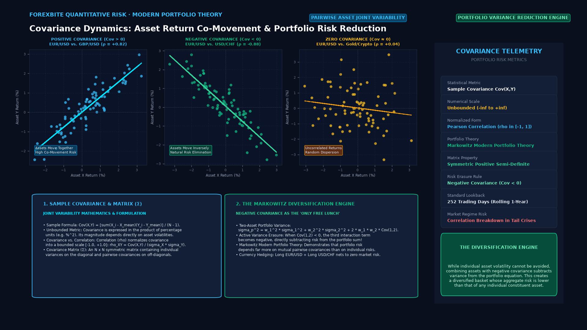Figure: Scatter plots of positive, negative, and zero asset return covariance, demonstrating the Markowitz Modern Portfolio Theory variance-reduction engine.

---

Key Takeaways

• Directional Co-Movement: Covariance reveals whether two assets move in the same direction ($> 0$) or opposite directions ($< 0$), but unlike correlation, it does not normalize the strength of the relationship.
• The Core Input for Portfolio Variance: In a two-asset portfolio, total portfolio variance depends not only on each asset’s individual volatility but critically on their pairwise covariance.
• Unbounded Scale: Because covariance is measured in the product of the assets’ percentage return units, its numerical value is unbounded and cannot be interpreted in isolation without knowing standard deviations.
• Risk Reduction via Negative Covariance: Combining currency pairs with negative covariance creates a portfolio whose aggregate volatility is significantly lower than the weighted average volatility of its individual assets.

---

Mathematical Formulation: Calculating Sample Covariance

Given two series of percentage price returns $X$ and $Y$ across $N$ trading periods, the sample covariance $\text{Cov}(X, Y)$ (or $\sigma_{XY}$) is computed as:

$$\text{Cov}(X, Y) = \frac{\sum_{i=1}^{N} (X_i - \bar{X})(Y_i - \bar{Y})}{N - 1}$$

Where:

• $X_i, Y_i$ = Daily percentage return of asset $X$ and asset $Y$ on day $i$
• $\bar{X}, \bar{Y}$ = Mean return of asset $X$ and asset $Y$ over the lookback window
• $N$ = Total number of observations

---

Covariance vs. Correlation: Critical Distinctions

Traders often conflate covariance with correlation. While inextricably linked, they perform fundamentally different analytical functions in quantitative modeling:

Analytical Property	Covariance ($\text{Cov}$)	Correlation ($r$ or $\rho$)
Statistical Definition	Measure of directional co-movement between two variables	Standardized, normalized measure of the strength and direction of linear co-movement
Scale / Range	Unbounded ($-\infty$ to $+\infty$)	Bounded strictly between -1.00 and +1.00
Measurement Units	Product of return units (e.g., $%^2$)	Dimensionless (pure ratio with no units)
Primary Utility	Mathematical engine in matrix algebra to compute total portfolio variance	Visual interpretation for traders evaluating pair relationships
Sensitivity to Volatility	Scales directly with asset volatility (higher volatility = larger covariance)	Completely independent of individual asset scale

$$\text{Correlation}(\rho) = \frac{\text{Cov}(X, Y)}{\sigma_X \cdot \sigma_Y} \iff \text{Cov}(X, Y) = \rho \cdot \sigma_X \cdot \sigma_Y$$

---

Modern Portfolio Theory: The Two-Asset Portfolio Variance Formula

Under Markowitz portfolio theory, when a trader allocates weight $w_1$ to Currency Pair 1 and weight $w_2$ to Currency Pair 2 ($w_1 + w_2 = 1.0$), the total portfolio variance $\sigma_p^2$ is:

$$\sigma_p^2 = w_1^2 \sigma_1^2 + w_2^2 \sigma_2^2 + 2 w_1 w_2 \text{Cov}(R_1, R_2)$$

Strategic Implication:

• If $\text{Cov}(R_1, R_2) > 0$, the covariance term adds risk to the portfolio.
• If $\text{Cov}(R_1, R_2) < 0$, the third term becomes negative, subtracting risk from the total portfolio.

---

Real-World Case Study: Constructing a Hedged Two-Pair Portfolio

A quantitative foreign exchange trader manages an institutional portfolio divided equally ($w_1 = 0.50$, $w_2 = 0.50$) between two active positions:

1. Asset 1 (Long EUR/USD): Annualized Volatility $\sigma_1 = 10%$ ($\sigma_1^2 = 0.0100$).
2. Asset 2 (Long USD/CHF): Annualized Volatility $\sigma_2 = 9%$ ($\sigma_2^2 = 0.0081$).

Scenario A: Historical Baseline (Negative Covariance)

Because EUR/USD and USD/CHF trade in strong inverse correlation ($\rho = -0.90$): $$\text{Cov}(R_1, R_2) = (-0.90) \times (0.10) \times (0.09) = -0.0081$$

Calculate Portfolio Volatility $\sigma_p$: $$\sigma_p^2 = (0.50)^2 (0.0100) + (0.50)^2 (0.0081) + 2(0.50)(0.50)(-0.0081)$$ $$\sigma_p^2 = 0.0025 + 0.002025 - 0.004050 = 0.000475$$ $$\sigma_p = \sqrt{0.000475} \approx 2.18%$$

Result: By pairing assets with negative covariance, total portfolio volatility collapses from an average of ~9.5% down to 2.18%—a massive 77% risk reduction achieved purely through mathematical diversification.

---

The Variance-Covariance Matrix in Institutional Risk Management

For institutional funds trading dozens of currency pairs, risk engines compile a Variance-Covariance Matrix ($\Sigma$):

$$\Sigma = \begin{bmatrix} \sigma_1^2 & \text{Cov}{1,2} & \text{Cov}{1,3} \ \text{Cov}{2,1} & \sigma_2^2 & \text{Cov}{2,3} \ \text{Cov}{3,1} & \text{Cov}{3,2} & \sigma_3^2 \end{bmatrix}$$

• The diagonal elements represent the individual variances of each asset.
• The off-diagonal elements represent the pairwise covariances.
• Risk algorithms multiply portfolio weight vectors by this matrix ($\sigma_p^2 = \mathbf{w}^T \Sigma \mathbf{w}$) to dynamically compute regulatory Value at Risk (VaR) and capital adequacy buffers under Basel III rules.

---

Frequently Asked Questions

Can covariance be negative?

Yes. Negative covariance indicates that when Asset A produces a return above its historical mean, Asset B tends to produce a return below its historical mean (inverse co-movement). In forex, EUR/USD and USD/CHF or AUD/USD and USD/CAD historically exhibit negative covariance.

Why do institutional traders use covariance instead of correlation?

Correlation is an intuitive, unitless number useful for human interpretation, but standard financial optimization algorithms (such as the quadratic programming models used to determine the Efficient Frontier) require covariance matrices because raw variances and unstandardized asset scales are necessary to calculate actual monetary portfolio risk.

Does a zero covariance mean two assets are completely independent?

No. A covariance of zero strictly indicates that there is no linear relationship between the two variables. It is statistically possible for two currency pairs to have a strong non-linear relationship (e.g., quadratic or regime-dependent co-movements during liquidity panics) while maintaining a measured linear covariance of zero.