Econometrics

What Is Econometrics?

Econometrics is the discipline that unifies economic theory, mathematical formulation, and statistical inference to analyze and quantify real-world financial phenomena. Coined by Norwegian economist Ragnar Frisch in the early 1930s, econometrics transforms qualitative economic hypotheses—such as “higher real interest rate differentials cause currency appreciation”—into rigorous, testable mathematical equations supported by empirical time-series data.

In institutional foreign exchange (FX) markets and quantitative asset management, econometrics serves as the bedrock for algorithmic trading, risk factor attribution, macroeconomic forecasting, and statistical arbitrage. Rather than relying on subjective chart observations, quantitative macro analysts employ econometric models to separate structural economic signals from random market noise.

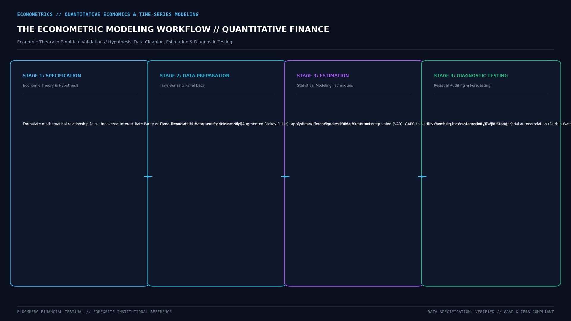Figure: Econometric modeling pipeline spanning Economic Hypothesis formulation, Data Stationarity testing (ADF), Model Estimation (OLS/ARIMA/VAR), Diagnostic Residual checking, and Out-of-Sample Forecasting.

---

Key Takeaways

• Empirical Validation: Econometrics provides the mathematical framework to confirm whether observed historical relationships between currency pairs and macroeconomic variables are statistically significant or merely coincidental.
• Handling Non-Stationarity: Raw FX prices exhibit non-stationary unit root behavior (random walk); econometrics utilizes log returns, first-differencing, and cointegration techniques to enable valid statistical modeling.
• Volatility Modeling via GARCH: Generalized Autoregressive Conditional Heteroskedasticity (GARCH) captures “volatility clustering”—the market reality where periods of turbulence are followed by turbulence, and calm periods by calm.
• Factor Attribution: Quantitative macro hedge funds utilize multi-factor econometric regressions to isolate pure alpha from common market betas like carry, momentum, and value.

---

Core Econometric Frameworks Used in Foreign Exchange

1. Ordinary Least Squares (OLS) & Multiple Regression

The starting point for testing economic relationships. In currency pricing, an analyst might model the spot exchange rate ($S_t$) against interest rate differentials ($\Delta i_t$), inflation differentials ($\Delta \pi_t$), and commodity price terms of trade ($TOT_t$):

$$Y_t = \beta_0 + \beta_1 X_{1t} + \beta_2 X_{2t} + \dots + \beta_k X_{kt} + \epsilon_t$$

Where:

• $Y_t$ is the dependent variable (e.g., change in AUD/USD exchange rate).
• $X_{kt}$ are the explanatory macroeconomic variables.
• $\beta_k$ are the estimated regression coefficients showing sensitivity.
• $\epsilon_t$ is the random error term, assumed to be white noise.

2. Time-Series Analysis: ARIMA

Autoregressive Integrated Moving Average (ARIMA) models project future price steps purely from historical serial dependencies:

• AR ($p$): Lags of the dependent variable itself.
• I ($d$): Degree of differencing required to achieve stationary data.
• MA ($q$): Lags of the forecast error terms.

3. Cointegration & Vector Error Correction Models (VECM)

Two non-stationary currency time series are cointegrated if a linear combination of them produces a stationary series. In FX pairs trading and statistical arbitrage, cointegration proves that two exchange rates share a true long-term equilibrium relationship that mean-reverts, allowing traders to exploit temporary pricing divergences without suffering from the spurious correlation common in standard OLS.

4. GARCH Volatility Modeling

Traditional statistics assume constant variance (homoskedasticity). Because FX volatility fluctuates violently around economic releases and geopolitics, GARCH($p, q$) models forecast time-varying volatility:

$$\sigma_t^2 = \omega + \sum_{i=1}^q \alpha_i \epsilon_{t-i}^2 + \sum_{j=1}^p \beta_j \sigma_{t-j}^2$$

Where $\sigma_t^2$ represents conditional variance, $\epsilon_{t-i}^2$ represents previous market shocks, and $\sigma_{t-j}^2$ represents prior forecast variance.

---

Comparative Analysis: Econometrics vs. Alternative Paradigms

Feature	Classical Econometrics	Machine Learning / Deep Learning	Technical Analysis
Foundational Theory	Deductive economic theory & formal statistical hypotheses	Inductive pattern discovery from data	Visual geometry and empirical price rules
Interpretability	Glass Box: Full transparency on $p$-values, $t$-statistics, and coefficients	Black Box: Complex non-linear neural weights; difficult to interpret	Subjective; varies across individual chartists
Overfitting Vulnerability	Low to moderate; constrained by theoretical priors	High; prone to memorizing noise in non-stationary markets	High; subjective cherry-picking of historical charts
Primary Domain	Macro factor modeling, equilibrium valuations, policy impact	High-frequency pattern recognition, order book dynamics	Short-term discretionary entry/exit timing

---

Practical Pitfalls in FX Econometric Modeling

1. Spurious Correlation: Running regressions on un-differenced, non-stationary exchange rate levels often yields deceptively high $R^2$ scores (>0.90) and high $t$-statistics even when no actual causal link exists between the series.
2. Structural Breaks: Central bank regime shifts (e.g., the Swiss National Bank abandoning the 1.20 EUR/CHF floor in 2015, or shifts from zero interest rates to rapid hiking cycles) instantly render historical regression parameters obsolete.
3. Endogeneity and Reverse Causality: While interest rates influence exchange rates, central banks simultaneously adjust interest rates in response to exchange rate fluctuations, biasing basic OLS estimates.

---

Frequently Asked Questions

Why do simple econometric models fail to accurately forecast spot FX rates?

As famously established by economists Richard Meese and Kenneth Rogoff in 1983, standard structural macroeconomic econometric models rarely outperform a simple random walk (naive persistence forecast) over horizons of 1 to 12 months. This occurs because exchange rates respond instantaneously to unpredictable news arrivals and institutional order flow shifts rather than smooth macroeconomic variables.

What is the Augmented Dickey-Fuller (ADF) test?

The ADF test is a statistical hypothesis test used to determine whether a given time series has a unit root (making it non-stationary) or is stationary. In currency modeling, traders must confirm that data series are stationary before running standard regression analyses to prevent spurious results.

How is econometrics used in retail automated trading?

Retail traders using algorithmic platforms like Python, R, or MetaTrader employ econometric functions to calculate rolling correlation matrices, historical value-at-risk (VaR), z-scores for mean-reverting pairs trading strategies, and dynamic volatility filters that adjust stop-loss buffers according to GARCH estimates.