Black-Scholes

What Is the Black-Scholes Model?

The Black-Scholes model (often referred to as the Black-Scholes-Merton or BSM model) is widely regarded as one of the most influential breakthroughs in the history of financial economics. Published in 1973 in the Journal of Political Economy by economists Fischer Black and Myron Scholes—and substantially expanded that same year by Robert C. Merton—the model provided the first mathematically rigorous formula for pricing derivative options contracts. In 1997, Scholes and Merton were awarded the Nobel Memorial Prize in Economic Sciences for their contribution (Fischer Black passed away in 1995).

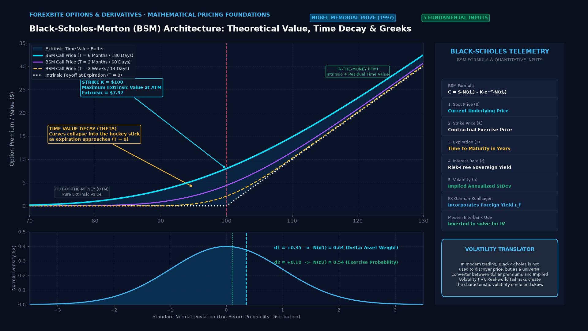
Prior to Black-Scholes, options trading was an imprecise, speculative craft governed by subjective intuition and inconsistent rule-of-thumb heuristics. By constructing a dynamic, continuously rebalanced riskless hedge consisting of the underlying asset and cash, Black and Scholes proved that the theoretical price of an option is uniquely determined without needing to forecast the expected future direction of the market.

The Five Fundamental Input Variables

The classical Black-Scholes formula determines an option’s theoretical premium based on five quantifiable market variables:

1. Underlying Asset Price ($S$): The current spot market price of the asset.
2. Strike Price ($K$): The predetermined price at which the option holder can buy (call) or sell (put) the asset.
3. Time to Expiration ($T$): The remaining duration until the option expires, expressed as a fraction of a 365-day year.
4. Risk-Free Interest Rate ($r$): The theoretical yield on default-free sovereign debt matching the option’s maturity (such as US Treasury yields).
5. Volatility ($\sigma$): The annualized standard deviation of the underlying asset’s logarithmic price returns. This is the only variable in the equation that cannot be directly observed on a live chart and must be estimated or inferred.

The mathematical formulation for a standard European call option ($C$) is expressed as:

$$ C = S \cdot N(d_1) - K \cdot e^{-rT} \cdot N(d_2) $$

Where $N(x)$ denotes the cumulative standard normal distribution function, and:

$$ d_1 = \frac{\ln(S/K) + (r + \frac{\sigma^2}{2})T}{\sigma \sqrt{T}} $$ $$ d_2 = d_1 - \sigma \sqrt{T} $$

The Garman-Kohlhagen Extension for Foreign Exchange

While the original 1973 model was formulated for non-dividend-paying stocks, it could not be applied directly to the global foreign exchange market without significant modification.

In currencies, both nations carry sovereign interest rates. Holding the base currency pays a foreign interest rate ($r_f$), while borrowing the quote currency incurs a domestic interest rate ($r_d$). In 1983, economists Mark Garman and Steven Kohlhagen adapted the BSM equation for currency options by treating the foreign risk-free interest rate as a continuous dividend yield.

The Garman-Kohlhagen formula for an FX call option is written as:

$$ C = S \cdot e^{-r_f T} \cdot N(d_1) - K \cdot e^{-r_d T} \cdot N(d_2) $$

Where: $$ d_1 = \frac{\ln(S/K) + (r_d - r_f + \frac{\sigma^2}{2})T}{\sigma \sqrt{T}} $$ $$ d_2 = d_1 - \sigma \sqrt{T} $$

In this foreign exchange formulation:

• If the foreign interest rate ($r_f$) rises relative to the domestic rate ($r_d$), the cost of holding the foreign currency increases, dampening the call option’s forward value.
• The formula perfectly incorporates the mechanics of Covered Interest Parity (CIP), ensuring that currency option pricing aligns with forward exchange rate curves.

The Greeks: Deriving Risk Sensitivities

A profound operational benefit of the Black-Scholes framework is the derivation of partial derivatives that quantify portfolio risk, universally known on trading desks as the Greeks:

• Delta ($\Delta$): The first derivative with respect to spot price ($\partial C / \partial S$). Delta measures the expected change in option premium for a one-unit change in the underlying currency. It defines the exact number of spot units required to establish a “delta-neutral” hedge.
• Gamma ($\Gamma$): The rate of change of Delta as the spot price moves ($\partial^2 C / \partial S^2$). Gamma reflects the stability of a hedge; high gamma requires frequent, expensive portfolio rebalancing.
• Vega ($\nu$): Sensitivity to shifts in implied volatility ($\partial C / \partial \sigma$). Vega indicates how many pips an option will gain or lose if market volatility expectations shift by 1.0%.
• Theta ($\Theta$): The rate of daily time decay ($\partial C / \partial T$). Theta quantifies the daily erosion of extrinsic value as expiration approaches.
• Rho ($\rho$): Sensitivity to shifts in domestic and foreign interest rates.

Real-World Limitations and the Volatility Smile

Although the Black-Scholes model revolutionized finance, its theoretical assumptions differ in important ways from real-world market behavior:

1. The Constant Volatility Fallacy

BSM assumes that volatility remains static throughout the life of the contract. In reality, volatility is dynamic and mean-reverting, clustering into tranquil periods followed by violent bursts of panic.

2. Log-Normal Distribution vs. “Fat Tails”

The model assumes that percentage price returns follow a Gaussian normal distribution. In real-world currency markets, extreme geopolitical crises, currency peg collapses, and liquidity freezes produce “fat tails” (leptokurtic distribution). Extreme multi-sigma events occur far more frequently in reality than BSM predicts.

3. The Volatility Smile and Skew

Because traders recognize that deep out-of-the-money options carry tail risk, market participants refuse to price all strikes using the same volatility. When implied volatility is plotted across various strike prices for a given maturity, it forms a U-shaped curve known as the volatility smile, or a tilted curve called the volatility skew.

How Modern FX Desks Actually Use Black-Scholes

On modern interbank dealing desks, the Black-Scholes equation is not used to tell traders what an option’s dollar price “should” be. Instead, dealers use the formula in reverse.

Because the market price of an option is determined by live supply and demand, dealers plug the market price, spot rate, strike, interest rates, and expiration date into the Black-Scholes equation to solve for the single missing variable: Implied Volatility (IV).

In institutional foreign exchange, vanilla options are not quoted in dollars or pips; they are quoted directly in volatility points (e.g., “1-month EUR/USD 25-delta risk reversal is trading at 7.25% vols”). The Black-Scholes equation acts as a universal quotation calculator that translates between volatility language and cash currency settlement.

Key Takeaways

• The Black-Scholes-Merton model is the foundational mathematical equation for calculating theoretical European option prices.
• Its five core inputs are Spot Price, Strike Price, Risk-Free Rate, Time to Expiration, and Volatility.
• The Garman-Kohlhagen extension adapts the model for foreign exchange by incorporating foreign and domestic interest rate differentials.
• The model mathematically derives the Greeks (Delta, Gamma, Vega, Theta, Rho), enabling precise institutional hedging.
• Real-world limitations—including fat tails and non-constant volatility—give rise to the volatility smile and volatility skew observed across options markets.

FAQ

Why can’t the standard Black-Scholes model price American options accurately? Black-Scholes assumes European exercise (the contract can only be exercised at the exact expiration timestamp). American options can be exercised at any point prior to expiration. Because the potential benefit of early exercise adds additional value, American options require numerical methods like the Binomial Tree or finite difference models.

What is implied volatility? Implied volatility is the expected future volatility of the underlying currency pair implied by the current market price of its options, calculated by backing out volatility from the Black-Scholes formula.

Why is volatility the most important variable in the model? Spot price, strike price, time to expiration, and interest rates are known, observable facts. Volatility is the only subjective input that requires forecasting, making options trading fundamentally a market for trading volatility rather than direction.